Kohns and Potjagailo (2025b) develop a Bayesian mixed-data-sampling framework (BMIDAS) that applies group-shrinkage priors (GIGG) to mixed frequency data, allows for estimation of latent (potentially slow-moving) trends and stochastic volatility with flexible hierarchical priors, and remains interpretable to the nowcaster due to the post-estimation sparsification algorithm which informs on variable importance over the nowcast cycle. The accompanying estimation code is released as the BMIDAS-GIGG toolbox (Kohns and Potjagailo 2025a).
So far this framework has been applied to UK data only. Small open (post-Soviet) economies such as Estonia differ from the United Kingdom in the composition of their indicator sets, in the length of their reliable statistical record (which tends to start reliably typically in the early 2000’s), and in the size and nature of shocks. Hence, in this case study, we put the Bayesian machinery of Kohns and Potjagailo (2025b) to the test by applying it to nowcasting Estonian q-o-q real GDP growth.
Next to the specific application to nowcasting to new data, this case study also functions as a resource to document the various nowcasting methods at the frontier of Bayesian modelling (and therefore might be often updated) as well as describe the data for a data base which will be publically available for the Estonian economy (and hopefully more in the future).
I summarise the aims of case study as as follows:
Apply the BMIDAS-GIGG framework to nowcasting Estonian real GDP growth.
Build a dataset suitable for nowcasting Estonian macroeconomic activity, assembled directly from source APIs, and archived as real-time vintages so that genuine real-time exercises become possible with time.1
Describe the frontier in Bayesian nowcasting models and benchmarking them on Estonian data. The model suite will be made publicly available.
Use the results to identify modelling avenues and to document what the estimates imply about Estonian macroeconomic dynamics.
2 Data description
2.1 Coverage and Role of Data
The core dataset contains 11 monthly indicators in 4 groups. Survey indicators cover manufacturing, construction and retail confidence together with consumer confidence and consumer price expectations. Real Activity is represented by the industrial production volume index and by accommodated tourists. Prices enter through the consumer and producer price indices. Energy enters through electricity and heat production. The target is quarterly GDP growth, chain-linked volume, seasonally and working-day adjusted.
The selection follows the standard nowcasting practice summarised in Bańbura et al. (2013), which is to combine a small set of timely soft indicators with the hard series that the target is mechanically related to. Survey balances are included because they are the only monthly series published within their own reference month, so they carry the entire information set in the earliest rounds of the release cycle. Industrial production is the single most important hard indicator for Estonia, where manufacturing dominates the goods-export base, and it is the series that the group prior selects most often at the end of the cycle. Consumer and producer prices enter as nominal counterparts that are considerably more timely than the volume data, a role documented for mixed-frequency models in Ghysels, Kvedaras, and Zemlys-Balevičius (2020). Electricity and heat production are high-frequency physical proxies for aggregate activity with a short publication delay. Accommodated tourists proxy the services side, which is otherwise unrepresented at monthly frequency because Estonia’s services turnover index only begins in 2020.
Two further blocks are introduced in Section 5. Financial market data are drawn from the European Central Bank Data Portal. Foreign activity is summarised by a single export-weighted index of industrial confidence in Estonia’s 4 largest goods-export destinations.
Code
core_series <-c("BCI_MANUF","BCI_CONSTR","BCI_RETAIL","CCI","CONS_PRICE_EXP","IP","TOURISTS","CPI","PPI","ELEC_PROD","HEAT_PROD")fin_series <-c("STOXX","EURIBOR3M","TERMSPREAD","EURUSD","LEND_RATE_EE")for_series <-c("FOREIGN_ICI")panel_of <-function(s) case_when(s %in% core_series ~"core", s %in% fin_series ~"financial", s %in% for_series ~"foreign")# Economic grouping, which is also the grouping the GIGG prior shrinks over.GROUPS <-c(BCI_MANUF ="SUR", BCI_CONSTR ="SUR", BCI_RETAIL ="SUR", CCI ="SUR",CONS_PRICE_EXP ="SUR", IP ="ACT", TOURISTS ="ACT",CPI ="PRI", PPI ="PRI", ELEC_PROD ="ENE", HEAT_PROD ="ENE",STOXX ="FIN", EURIBOR3M ="FIN", TERMSPREAD ="FIN", EURUSD ="FIN",LEND_RATE_EE ="FIN", FOREIGN_ICI ="FOR")tibble(series =c(core_series, fin_series, for_series)) %>%mutate(panel =panel_of(series)) %>%left_join(labels %>%distinct(series, .keep_all =TRUE), by ="series") %>%left_join(manifest %>%select(series, first_obs, last_obs), by ="series") %>%mutate(source =case_when( series =="FOREIGN_ICI"~"Eurostat, export-weighted", series =="TERMSPREAD"~"ECB, derived",TRUE~recode(source, statee ="Statistics Estonia", ecb ="ECB Data Portal",eurostat ="Eurostat", oecd ="OECD")),first_obs =format(as.Date(first_obs), "%Y-%m"),last_obs =format(as.Date(last_obs), "%Y-%m")) %>%# TERMSPREAD and FOREIGN_ICI are derived inside the export step rather than fetched, so# they carry no registry row. Their spans are the intersection of their inputs.mutate(group = GROUPS[series],table =coalesce(table, c(TERMSPREAD ="FM", FOREIGN_ICI ="ei_bssi_m_r2")[series]),first_obs =coalesce(first_obs, c(TERMSPREAD ="1994-01", FOREIGN_ICI ="2000-01")[series]),last_obs =coalesce(last_obs, c(TERMSPREAD ="2026-07", FOREIGN_ICI ="2026-07")[series])) %>%select(Series = series, Group = group, Panel = panel, Source = source, Table = table,From = first_obs, To = last_obs) %>%kable()
Table 1: Indicators, sources and coverage. Group codes are SUR surveys, ACT real activity, PRI prices, ENE energy, FIN financial, FOR foreign. Panel indicates the indicator set in which each series is used.
Series
Group
Panel
Source
Table
From
To
BCI_MANUF
SUR
core
OECD
OECD.SDD.STES,DSD_STES@DF_BTS,4.0
1992-04
2026-04
BCI_CONSTR
SUR
core
OECD
OECD.SDD.STES,DSD_STES@DF_BTS,4.0
1994-04
2026-04
BCI_RETAIL
SUR
core
OECD
OECD.SDD.STES,DSD_STES@DF_BTS,4.0
1995-01
2026-04
CCI
SUR
core
OECD
OECD.SDD.STES,DSD_STES@DF_CS,4.0
1992-10
2026-04
CONS_PRICE_EXP
SUR
core
OECD
OECD.SDD.STES,DSD_STES@DF_CS,4.0
1993-04
2026-04
IP
ACT
core
Statistics Estonia
TO0053
2000-01
2026-06
TOURISTS
ACT
core
Statistics Estonia
TU121
1996-01
2026-06
CPI
PRI
core
Statistics Estonia
IA002
1998-01
2026-07
PPI
PRI
core
Statistics Estonia
IA039
2002-01
2026-07
ELEC_PROD
ENE
core
Statistics Estonia
KE20
2000-01
2026-06
HEAT_PROD
ENE
core
Statistics Estonia
KE20
2000-01
2026-06
STOXX
FIN
financial
ECB Data Portal
FM
1990-01
2026-07
EURIBOR3M
FIN
financial
ECB Data Portal
FM
1994-01
2026-07
TERMSPREAD
FIN
financial
ECB, derived
FM
1994-01
2026-07
EURUSD
FIN
financial
ECB Data Portal
EXR
1999-01
2026-07
LEND_RATE_EE
FIN
financial
ECB Data Portal
MIR
2000-01
2026-06
FOREIGN_ICI
FOR
foreign
Eurostat, export-weighted
ei_bssi_m_r2
2000-01
2026-07
Seasonal adjustment is handled series by series and the treatment differs across the panel. Industrial production is calendar and seasonally adjusted by Statistics Estonia at source and is passed through unchanged. Tourists, the consumer and producer price indices, and electricity and heat production are published unadjusted, and we adjust them ourselves by seasonal-trend decomposition using loess. The survey balances are also adjusted by us rather than at source, for the reason set out below. Financial series and the foreign activity index are not seasonally adjusted, the former because financial prices carry no seasonality, the latter because Eurostat publishes it already adjusted.
One data quirk requires separate treatment. Estonia’s business and consumer survey moved from the Estonian Institute of Economic Research to Statistics Estonia in May 2026, and publication of the Estonian data by the European Commission has been suspended in the interim. The historical and current tranches therefore come from different producers and there is no overlap on which to calibrate the joint series. Both halves are taken unadjusted, and a single pass of X-13ARIMA-SEATS with a user-specified level shift at the break (May 2026) performs the seasonal adjustment and the level correction in one go. Since the level shift is estimated from very few post-break observations, the post shift survey observations may carry more uncertainty than the historical ones. As more data accumulates, we will be able to adjust this procedure further.
2.2 Stylised release calendar
The models we propose in Kohns and Potjagailo (2025b) are based on the MIDAS methodology. This is a direct nowcasting technique (see Bańbura et al. (2013)), where the models are re-estimated at the identified data publication days within each nowcast cycle. In our case, we stylise this release calendar to 15 points inside each quarter. At each point the model observes only what would genuinely have been published by then which depends on a variable’s publication delay. The publication delay records how many months after a reference month an observation appears, where 0 means within the reference month itself. Slot in the below refers to the sequencing group in which the data arrive (this is often necessary to include since also in real time, many data series, often by the same provider, are published together).
Code
# Round to calendar position, verified against the emission order of calendar_gen in the# toolbox. The first 3 months of the target quarter carry 4 rounds each and the month# after the quarter ends carries 3, because the surveys are complete by then and so# trigger no further round. Within-month rounds are stylised as evenly spaced, 7 days# apart, starting at the beginning of the month. The flash release arrives about 29 days# after the quarter ends, which fixes the day count reported in @fig-calendar.round_pos <-tibble(round =1:15,quarter =c(rep("Quarter t", 12), rep("Quarter t+1", 3)),month =c(rep("M1", 4), rep("M2", 4), rep("M3", 4), rep("M1", 3)),days_to_flash =c(120, 113, 106, 99, 90, 83, 76, 69, 60, 53, 46, 39, 29, 22, 15))calendar %>%rename(Indicator = indicator, Delay = pubdelay, Slot = pubseq) %>%kable(format ="html",col.names =c("Indicator", "Delay", "Slot", paste0("r", round_pos$round))) %>%kable_styling(full_width =FALSE, bootstrap_options =c("striped", "condensed")) %>%add_header_above(c(" "=3, "M1"=4, "M2"=4, "M3"=4, "M1"=3)) %>%add_header_above(c(" "=3, "Quarter t"=12, "Quarter t+1"=3))
Table 2: Stylised release calendar. Cells give the number of monthly lags observed at each release round. The header rows give the quarter, the calendar month inside that quarter, and the release round.
Quarter t
Quarter t+1
M1
M2
M3
M1
Indicator
Delay
Slot
r1
r2
r3
r4
r5
r6
r7
r8
r9
r10
r11
r12
r13
r14
r15
BCI_MANUF
0
1
4
4
4
4
5
5
5
5
6
6
6
6
6
6
6
BCI_CONSTR
0
1
4
4
4
4
5
5
5
5
6
6
6
6
6
6
6
BCI_RETAIL
0
1
4
4
4
4
5
5
5
5
6
6
6
6
6
6
6
CCI
0
1
4
4
4
4
5
5
5
5
6
6
6
6
6
6
6
CONS_PRICE_EXP
0
1
4
4
4
4
5
5
5
5
6
6
6
6
6
6
6
IP
-2
5
1
1
1
2
2
2
2
3
3
3
3
4
4
4
5
TOURISTS
-2
5
1
1
1
2
2
2
2
3
3
3
3
4
4
4
5
CPI
-1
2
2
3
3
3
3
4
4
4
4
5
5
5
6
6
6
PPI
-1
4
2
2
3
3
3
3
4
4
4
4
5
5
5
6
6
ELEC_PROD
-1
4
2
2
3
3
3
3
4
4
4
4
5
5
5
6
6
HEAT_PROD
-1
4
2
2
3
3
3
3
4
4
4
4
5
5
5
6
6
Surveys are published without any delay and all 6 lags are available by round 9. Industrial production, with its two-month delay, has only 1 lag available at round 1 and still only 5 at round 15. The third month of the target quarter is therefore never observed for hard activity before the GDP flash estimate arrives.
Two features of Table 2 deserve comment. Survey arrive with a delay of 0 because Statistics Estonia now publishes within the reference month, on the 23rd. The quarterly target carries a delay of minus 1 because we consider the flash estimate to be the target for estimation. Since the flash estimate is not available for the entire evaluation period considered, we use the final vintages of GDP where available (until 2025) and use the flash estimates for GDP values of Q1-Q2 2026.
2.2.1 Estimation and evaluation windows
Code
tibble(Item =c("Monthly sample", "Quarterly sample", "First nowcast quarter","Training quarters before the first nowcast", "Evaluation quarters","Release rounds per quarter", "Monthly lags", "Scored through","Conditioning only, not scored"),Value =c("2000M01 to 2026M09", "2000Q1 to 2026Q3", "2008Q1","31", "74", "15", "6", "2025Q4","2026Q1 to 2026Q3")) %>%kable()
Table 3: Estimation and evaluation windows.
Item
Value
Monthly sample
2000M01 to 2026M09
Quarterly sample
2000Q1 to 2026Q3
First nowcast quarter
2008Q1
Training quarters before the first nowcast
31
Evaluation quarters
74
Release rounds per quarter
15
Monthly lags
6
Scored through
2025Q4
Conditioning only, not scored
2026Q1 to 2026Q3
The estimation window expands. At each evaluation quarter the model is re-estimated on all data up to that quarter, and then filtered through each of the 15 release rounds. Nothing after the quarter being nowcast enters the estimation sample.
The last three quarters require a separate convention. Their outturn is either a flash estimate or not yet published, so they are used as conditioning information for the live nowcast (this is what we call the nowcast for the next arriving quarter, which is of now Q3-2026) but are excluded from every score reported below. Mixing a first-release vintage into the scored sample would compare models against a target that is itself subject to revision, and over the 16 quarters where both are available the flash and the final vintage differ by an average of 1 percentage point on a year-on-year basis.
Figure 1 summarises the same information visually, with indicators grouped by their release group. The numbers in each block tells us how many monthly lags (out of 6) are available to the modeler. For example at round 1, 120 days until GDP comes out, we have access to the first month of the reference quarter’s surveys, as well as all surveys of the previous quarter, which makes for the availability of 4 lags of surveys which can be fed to the model.
Note that the choice to model with a total of 6 monthly lags is a modeling decision not a data availability issue. We could have for example used 12 lags in order to always use a year’s worth of monthly data (this however, has been tested and did not improve nowcasting performance).
Code
# The release groups are the publication slots of @tbl-calendar.SLOT_LABELS <-c(`1`="Surveys", `2`="Consumer prices",`4`="Producer prices, energy", `5`="Real activity")cal_long <- calendar %>%pivot_longer(starts_with("r"), names_to ="round", values_to ="lags") %>%mutate(round =as.integer(sub("^r", "", round)),# Keep the publication order of the calendar rather than sorting alphabetically.indicator =factor(indicator, levels =rev(calendar$indicator)),group =factor(SLOT_LABELS[as.character(pubseq)], levels = SLOT_LABELS)) %>%left_join(round_pos, by ="round")# Column labels carry the countdown to the flash release, which falls by 7 days within a# month and then jumps at the month boundary.col_labels <-with(round_pos,paste0(round, "\n", ifelse(quarter =="Quarter t", "t", "t+1"), " ", month, "\n", days_to_flash, "d"))ggplot(cal_long, aes(x =factor(round), y = indicator, fill = lags)) +geom_tile(colour ="white", linewidth =1.2) +geom_text(aes(label = lags, colour = lags >3), size =3.4, show.legend =FALSE) +facet_grid(group ~ ., scales ="free_y", space ="free_y", switch ="y") +scale_x_discrete(position ="top", labels = col_labels, expand =c(0, 0)) +scale_colour_manual(values =c(`TRUE`="white", `FALSE`="grey20")) +scale_fill_gradient(low ="#E8F0F5", high ="#1F6F8B", limits =c(0, 6),breaks =c(0, 3, 6), name ="months of 6") +labs(title ="Data availability across the release cycle",subtitle =paste("Months of the 6-month lag window observed at each round.","Column labels give the round, its calendar month,","\nand the approximate number of days until the GDP flash release."),x =NULL, y =NULL) +guides(fill =guide_colourbar(barwidth =8, barheight =0.6, title.vjust =1)) +theme_minimal(base_size =11) +theme(panel.grid =element_blank(),strip.placement ="outside",strip.text.y.left =element_text(angle =0, hjust =1, size =10),axis.text.x.top =element_text(size =8.5, lineheight =1.15),axis.text.y =element_text(family ="mono", size =8.5),legend.position ="bottom",plot.title =element_text(face ="bold"),plot.subtitle =element_text(colour ="grey30", size =9))
Figure 1: Months of the 6-lag window observed by each indicator at each release round. Column labels give the round, the calendar month it falls in, and the approximate number of days until the GDP flash release.
2.3 Missing observations
Missing values arise in 3 ways. Producer prices begin in 2002 and require backfilling over 2000 and 2001. Trade series begin in 2004, when Intrastat replaced customs collection on accession to the European Union. Financial series contain scattered gaps where the underlying return was suppressed for confidentiality.
The toolbox of Kohns and Potjagailo (2025b) imputes missing entries by principal-components expectation maximisation on the monthly panel before the release calendar is applied, following Stock and Watson (2002), with the treatment of arbitrary missing patterns as in Bańbura and Modugno (2014). Since the evaluation period begins after any missing values existence, imputed values are never used for nowcast evaluation. Imputed cells that predate the first evaluation quarter still shape the parameter estimates of the early expanding-window fits, and the trade and financial blocks should be read with that in mind.
3 Model description
3.1 The BMIDAS-GIGG model
Let y_t denote quarterly GDP growth in quarter t and let x^{(m)}_{i,t} denote monthly indicator i at monthly lag m = 0, \dots, M-1 within the window, with m = 0 the most recent month. The observation equation is
Here \tau_t is the stochastic trend, h_t the log-variance of the observation equation, and g_t the log-variance of the trend innovation, so the trend itself is allowed to move at a time-varying rate. The scale parameters \omega_g and \omega_h govern how much time variation the trend and the volatility admit, and the model nests a static trend at \omega_g = 0 and a homoskedastic observation equation at \omega_h = 0. This case study places penalised complexity priors (Simpson et al. 2017) on both, in the non-centred parameterisation of Equation 2. The penalised complexity prior places an exponential penalty on the Kullback-Leibler distance from the simpler model in which the scale is zero, which is a static trend and a homoskedastic observation equation. This shrinks toward the simpler model without bounding the scale away from zero, which is the failure mode of the conditionally conjugate inverse-gamma alternative.
The regression coefficients receive the group inverse-Gamma gamma prior (GIGG) as proposed in Kohns and Potjagailo (2025b) . Each indicator forms a group (of lags), to which 3-tiered hierarchical shrinkage is applied: 1) on the entire collection of groups, i.e., global shrinkage (\nu) , 2) on the indicator group level, shrinking the collection of monthly lags jointly (\gamma_i) , 3) on the lag level which allows to estimate how correlated individual and group-wise shrinkage is (\lambda_{i,m}). Kohns and Potjagailo (2025b) show that this prior significantly improves inference and nowcasting compared to popular shrinkage priors. Writing \beta_{(i)} for the coefficient block of indicator i, the prior takes the following form:
While it would be possible to set the hyperparameters (a_g,b_g) for each indicator separately, we follow the recommendations of Kohns and Potjagailo (2025b) by estimating a_g via a hierarchical prior and set b_g=0.5 in order to push the posterior on \beta_{(i)} toward high intra group correlation.
The group scale \gamma_i controls whether an indicator enters at all and the local scales \lambda_{i,m} control the shape of its lag profile. Finally, posterior draws are then sparsified by group signal-adaptive variable selection proposed in Kohns and Potjagailo (2025b), which maps the continuous posterior to a set of exact zeros and yields the inclusion probabilities reported in Section 4.3. This allows interpreting the high-dimensional poster in terms of which indicator is most probably to influence the predictions.
3.2 The lag polynomial
An unrestricted specification assigns one coefficient to every indicator and lag, which here would be 66 coefficients for 11 indicators over 6 months. The Almon restriction (Almon 1965) replaces the free lag profile with a low-order polynomial which is gradient and end point restricted peter out smoothly to zero with the last lag. The restriction imposes smoothness within an indicator’s lag profile and allows Equation 3 to go from 6 coefficients per group to only 2.
Concretely, the coefficient on lag m of indicator i is written as a polynomial in the lag index,
which are the endpoint and gradient restrictions. The coefficient on the most distant lag is zero and the profile approaches it with zero slope, so the lag structure tapers off smoothly rather than being truncated. With M = 6 and a third-degree polynomial, two restrictions leave P = 2 free parameters \theta_{i,1} and \theta_{i,2} per indicator, which is why each group in Equation 3 has two members.
The practical consequence is that the prior shrinks a shape rather than 6 unrelated numbers. Figure 2 shows the two basis functions and a set of admissible profiles. The restriction is not as tight as it first appears. Combinations of the two functions deliver monotone decay at different speeds, sign reversals, and hump-shaped profiles that peak one or two months back, which is the shape one would expect for an indicator that leads the target.
Figure 2: The restricted Almon basis and the coefficient profiles it can express.
3.3 Model Overview
Code
tibble(Model =c("GIGG-SV-trend", "GIGG-SV", "GIGG", "PCA-MIDAS", "DFM"),Trend =c("random walk, PC prior", "none", "none", "none", "random walk"),`Observation volatility`=c("stochastic, PC prior", "stochastic, PC prior","homoskedastic", "homoskedastic", "stochastic"),`Lag treatment`=c("Almon", "Almon", "Almon", "principal components","state-space aggregation"),Shrinkage =c("GIGG", "GIGG", "GIGG", "GIGG on components, no sparsification", "none")) %>%kable()
Table 4: Estimated specifications. All BMIDAS-GIGG variants use the Almon restriction and 6 monthly lags.
Model
Trend
Observation volatility
Lag treatment
Shrinkage
GIGG-SV-trend
random walk, PC prior
stochastic, PC prior
Almon
GIGG
GIGG-SV
none
stochastic, PC prior
Almon
GIGG
GIGG
none
homoskedastic
Almon
GIGG
PCA-MIDAS
none
homoskedastic
principal components
GIGG on components, no sparsification
DFM
random walk
stochastic
state-space aggregation
none
We test 3 BMIDAS-GIGG variants which form a nested sequence of model components. GIGG-SV-trend includes a stochastic trend and stochastic volatility (h_t,g_t), GIGG-SV drops the trend (\tau_t = \bar{\tau}), and GIGG drops both.
Two models from outside the framework serve as comparators.
PCA-MIDAS takes the unrestricted MIDAS design of every monthly lag available at a given release round and replaces it with its leading 4 principal components, recomputed at every round and every estimation window on that window’s data alone. The components are extracted from the correlation matrix, because the design mixes percentage changes with standardised survey balances and an unstandardised extraction would track whichever block carries the larger variance. No trend and no stochastic volatility are applied. The approach is the factor-MIDAS of Marcellino and Schumacher (2010), which extracts principal components from a ragged-edge monthly panel and regresses the quarterly target on them, and it is closely related to the daily-frequency factor constructions of Andreou, Ghysels, and Kourtellos (2013).
We do not sparsify the component loadings. Doing so was tested and it degenerates. Group sparsification is a statement about which indicators enter, and once the regressors are principal components there are no indicator groups left to select.
DFM is the Bayesian dynamic factor model of the Federal Reserve Bank of New York (Federal Reserve Bank of New York, Research and Statistics Group 2024), following Drechsel, Antolín-Díaz, and Petrella (2024) and in the tradition of Bańbura et al. (2013). Similar to the full BMIDAS-GIGG model, it estimates a random-walk trend in mean, and stochastic volatility, however for both the factor and the idiosyncratic innovations. Additionally, it includes estimation of a discrete outlier term which Drechsel, Antolín-Díaz, and Petrella (2024) have shown to significantly improve computational stability when outliers are contained in the data set, as well as improve nowcasting performance during crisis times. The DFM frameworks largest departure from the MIDAS framework is that it estimates the model at the lowest available frequency, here the monthly frequency, and uses the joint model over indicators and the target to interpolate any missing data at time of estimation with the system. While convenient for drawing inference on unobservable targets such as monthly GDP, the previous literature has shown that whether the DFM or MIDAS framework dominates, is often a factor of the available time-series length (often the DFM requires many more observations in order to enable accurate inference on unknown states) as well as whether the data generating process for the target is truly sparse or dense. In the latter case, it has been shown (Giannone, Lenza, and Primiceri (2021)) that factor and dynamic factor models can outperform shrinkage methods, while in the former case, estimating with shrinkage priors can outperform (additionally mutli-step ahead forecasts are often better with the full system DFM models compared to MIDAS models). Quarterly aggregation follows the Mariano-Murasawa weighting. It is estimated on the same 11 indicators and filtered through the same release calendar, so the information sets are identical by construction.
4 Core results
The evaluation covers 74 quarters from 2008Q1, with 31 quarters of training data before the first nowcast. Subsamples are the global financial crisis to the end of 2009, a tranquil period from 2010 to 2019, and the pandemic period from 2020. Quarters whose outturn is available only as a flash estimate are used as conditioning information.
Three scores are reported. Write y_t for the outturn, \hat{y}_t for the predictive mean and F_t for the predictive distribution function at quarter t.
The root mean squared forecast error evaluates the point forecast only,
All 3 are negatively oriented, so lower is better throughout. The CRPS and the WQS are proper scoring rules in the sense of Gneiting and Raftery (2007), so they are minimised in expectation by the true predictive distribution. The RMSFE rewards only the central tendency, which is why a model can improve on it while worsening the density.
4.1 Accuracy across the release cycle
Figure 3: Root mean squared forecast error, continuous ranked probability score and tail-weighted quantile score across the 15 release rounds, by subsample.
Table 5: Scores averaged over release rounds. Lower is better.
Model
Metric
Full
GFC
Tranquil
Pandemic
GIGG-SV-trend
RMSFE
1.908
4.750
0.923
1.896
GIGG-SV
RMSFE
1.939
4.534
0.855
1.787
GIGG
RMSFE
1.966
4.874
0.937
1.802
PCA-MIDAS
RMSFE
2.205
5.363
0.979
2.277
DFM
RMSFE
2.043
4.470
0.858
1.746
GIGG-SV-trend
CRPS
1.163
3.118
0.744
1.291
GIGG-SV
CRPS
1.000
2.829
0.611
1.114
GIGG
CRPS
0.997
2.477
0.667
1.113
PCA-MIDAS
CRPS
1.081
2.846
0.659
1.268
DFM
CRPS
0.929
3.111
0.512
0.989
GIGG-SV-trend
WQS
0.368
1.140
0.210
0.405
GIGG-SV
WQS
0.358
1.228
0.193
0.379
GIGG
WQS
0.372
1.048
0.253
0.375
PCA-MIDAS
WQS
0.421
1.138
0.267
0.468
DFM
WQS
0.391
1.403
0.205
0.405
Code
dm <-d("dm_vs_benchmark.csv")# The toolbox convention stars improvements only. Reporting deteriorations unmarked would# be misleading here, because several are significant at well below the 1% level.# They are marked in parentheses.sig <-function(p) ifelse(is.na(p), "", ifelse(p <0.01, "***", ifelse(p <0.05, "**",ifelse(p <0.10, "*", ""))))fmt <-function(ratio, pval) { mark <-sig(pval)ifelse(is.na(ratio), "",ifelse(ratio <1,paste0("<strong>", sprintf("%.3f", ratio), mark, "</strong>"),paste0(sprintf("%.3f", ratio), ifelse(mark =="", "", paste0("(", mark, ")")))))}dm %>%filter(spec %in% CORE, subsample %in%c("Full","GFC","Tranquil","Pandemic")) %>%mutate(cell =fmt(ratio, pval),metric =recode(metric, rmsfe ="RMSFE", crps ="CRPS", wqs ="WQS")) %>%select(spec, subsample, metric, cell) %>%pivot_wider(names_from = subsample, values_from = cell) %>%arrange(factor(metric, levels =c("RMSFE","CRPS","WQS")),factor(spec, levels = CORE)) %>%rename(Model = spec, Metric = metric) %>%kable(escape =FALSE)
Table 6: Scores relative to the GIGG benchmark. Values below 1 indicate an improvement and are shown in bold. Significance is from the Diebold-Mariano test with the Harvey-Leybourne-Newbold correction, on the same loss differentials the toolbox uses, with * p<0.10, ** p<0.05, *** p<0.01. Bare stars mark significant improvements and stars in parentheses mark significant deteriorations.
Model
Metric
Full
GFC
Tranquil
Pandemic
GIGG-SV-trend
RMSFE
0.970
0.974*
0.985
1.052(**)
GIGG-SV
RMSFE
0.986
0.930***
0.913***
0.992
GIGG
RMSFE
1.000
1.000
1.000
1.000
PCA-MIDAS
RMSFE
1.121(***)
1.100(***)
1.045
1.264(***)
DFM
RMSFE
1.012
0.868
0.883**
0.929
GIGG-SV-trend
CRPS
1.167(***)
1.258(***)
1.115(***)
1.160(***)
GIGG-SV
CRPS
1.003
1.142(***)
0.916***
1.001
GIGG
CRPS
1.000
1.000
1.000
1.000
PCA-MIDAS
CRPS
1.084(***)
1.149(***)
0.987
1.139(***)
DFM
CRPS
0.939
1.275
0.746***
0.893*
GIGG-SV-trend
WQS
0.987
1.088(*)
0.832***
1.079(***)
GIGG-SV
WQS
0.960***
1.172(***)
0.762***
1.011
GIGG
WQS
1.000
1.000
1.000
1.000
PCA-MIDAS
WQS
1.131(***)
1.086(***)
1.058(***)
1.249(***)
DFM
WQS
1.032
1.374
0.778***
1.025
Before turning to the differences between models, note the feature they share. In Figure 3 every score on average declines as the release round advances. This is the minimum one should require of a nowcasting exercise as it indicated that the indicators carry information about the target and that the release calendar orders that information in a coherent way (and that the correlation structure to the target behaves in a somewhat linear way). A flat or rising profile may indicate that the data are uninformative or that the calendar is misspecified.
Three results stand out.
First, the ordering of the 3 GIGG variants differs between the point forecast and the density, and the Diebold-Mariano tests in Table 6 show the two comparisons carry very different weight. On the point forecast, GIGG-SV improves significantly on the homoskedastic GIGG in the crisis subsample, at a ratio of 0.930 with p below 0.01, and in the tranquil period, at 0.913 with p below 0.01. Over the full sample the point-forecast differences among the 3 are not significant.
On the density the ranking reverses and the reversal is significant. GIGG-SV-trend is worse than GIGG on the continuous ranked probability score over the full sample, at a ratio of 1.167 with p below 0.01, and worse again in the crisis subsample at 1.258. GIGG-SV is indistinguishable from GIGG over the full sample, at 1.003 with p of 0.78, but significantly worse in the crisis subsample at 1.142. A homoskedastic model produces bands of uniform width, and over a sample containing one very large observation this turns out to be a better probabilistic description for that outturn than a model that widens its bands only after the fact. Adding the trend on top costs accuracy on both criteria and is the least attractive of the 3.
Second, the dynamic factor model attains the lowest continuous ranked probability score over the full sample, but the margin over GIGG is not significant, at a ratio of 0.939 with p of 0.46. Its advantage is concentrated in the tranquil period, where the ratio of 0.746 is significant at the 1% level, and it reverses in the crisis subsample, where it scores 1.275 against GIGG.
The mechanism is visible in the decomposition reported in the appendix. The model’s stochastic volatility paths are close to constant, and its random-walk trend spans a range of only 0.022 to 0.030 percentage points over 26 years. Both crises are absorbed almost entirely by the discrete outlier component, which is a multiplicative scale on the innovation variance. That scale sits at 1 in 319 of 321 months and fires exactly twice, at 2008Q4 with a multiple of 4.6 and at 2020Q3 with a multiple of 3.6. The factor model therefore handles the crisis episodes by inflating variance at two points rather than by tracking the level, and its cycle correspondingly picks up less of the variation in growth than the MIDAS models do, resulting in worse overall RMSFE. This is a different mechanism from the one the GIGG variants use, and it is why the factor model looks strong on a density score in quiet periods and weak in the crisis.
Third, PCA-MIDAS is the weakest specification, and unlike the differences among the GIGG variants this one is unambiguous. It is worse than GIGG on every metric in every subsample, and significantly so at the 1% level throughout, with a full-sample point-forecast ratio of 1.121. The Almon restriction and the principal-components reduction impose different structures. The Almon polynomial restricts the lag profile within each indicator, as Figure 2 illustrates, whereas principal components impose a common low-rank structure across indicators and lags and discard indicator-specific timing. On this panel the former is clearly the more useful restriction.
Figure 4: Predictive median and 68% and 90% bands against realised GDP growth, by model and release round.
Figure 4 shows the source of the score differences. All 5 models track the tranquil period closely and all 5 miss the 2008Q4 and 2020Q2 troughs. The differences between models are differences in how much uncertainty they attach to those misses and therefore how much the conditional mean is able to adjust.
Table 7: Mean width of the 90% predictive interval, in percentage points, by release round.
Model
round 1
round 3
round 5
round 9
round 15
GIGG-SV-trend
8.47
6.35
6.01
5.80
5.68
GIGG-SV
7.18
6.02
5.83
5.74
5.55
GIGG
7.34
6.15
5.81
5.96
5.42
PCA-MIDAS
7.47
6.56
6.36
5.99
5.91
DFM
4.38
4.43
4.53
4.39
4.35
Uncertainty narrows as information accrues, which is the density counterpart of the score profile noted above. For the 4 MIDAS-family specifications the 90% interval contracts by between a fifth and a quarter between the first and the last round. The dynamic factor model is the exception. Its interval is both much narrower throughout and essentially flat across the cycle, moving from 4.38 to 4.35 percentage points. A model whose predictive uncertainty does not respond to the arrival of 3 additional months of hard data is not learning from the release calendar in the way the others are, and this is the same limitation that flatters its density scores. The PCA-MIDAS interval is the widest of the MIDAS family at every round, which alongside its point-forecast performance is the second reason to prefer the Almon restriction on this panel.
4.2 Trend, cycle and volatility
Figure 5: Posterior median and 90% credible bands for the trend, cycle and observation volatility at the final release round.
The trend estimated by GIGG-SV-trend is close to constant at approximately 0.4% per quarter over the entire sample, with a credible band that never excludes a flat trend after 2011. This is consistent with the score evidence, where dropping the trend costs little on the point forecast, however improves density nowcasts because it allows to more flexibly model the uncertainty propagation.
The cycle carries essentially all of the variation and the two models agree on it closely. The observation volatility rises sharply in 2008 and 2009, falls to a low and stable level through the 2010s, and rises again through 2020 to 2022 without approaching the crisis peak. GIGG-SV assigns systematically higher volatility than GIGG-SV-trend in the crisis episode, which is the expected consequence of removing the trend. Variation that the trend would otherwise absorb is reallocated to the variance of the observation equation.
4.3 Inclusion probabilities
Figure 6: Posterior group inclusion probability by indicator and release round, pre-pandemic and pandemic periods.
Table 8: Group inclusion probabilities at the final release round, full sample.
Indicator
GIGG-SV-trend
GIGG-SV
GIGG
BCI_MANUF
0.86
0.88
0.74
IP
0.91
0.70
0.97
CPI
0.66
0.59
0.77
BCI_CONSTR
0.54
0.47
0.75
CONS_PRICE_EXP
0.86
0.47
0.70
CCI
0.56
0.42
0.60
HEAT_PROD
0.33
0.27
0.36
TOURISTS
0.34
0.25
0.34
BCI_RETAIL
0.55
0.16
0.29
ELEC_PROD
0.19
0.15
0.24
PPI
0.20
0.14
0.22
As indicated above, we use a sparsification algorithm proposed in Kohns and Potjagailo (2025b) in order to identify which indicator over the nowcast cycle influences the nowcasts the most. The result of applying the sparsification algorithm is a number for every nowcast period for each indicator between 0 and 1 (hence, we often refer to it in the paper as an inclusion probability). The closer this number gets to 1, the more important that indicator is in forming the nowcast.
The 3 BMIDAS-GIGG variants agree on which indicators matter. Industrial production and manufacturing confidence carry the highest probabilities at the final release round, and the consumer price index and consumer price expectations follow. Energy production and tourism are selected least often. This is a coherent reading for an economy in which manufacturing dominates the goods-export base.
The pattern across the release cycle is more informative than the level. At early rounds, when no hard activity data are available, the survey and price groups carry the entire signal. Industrial production enters only from the rounds at which its first month becomes observable, and its probability then rises monotonically. The model reallocates weight from soft to hard information as the latter arrives, which is the behaviour the group structure was designed to produce.
Interestingly, there is fairly little difference in the inclusion probabilities before and during the pandemic, whereas for the UK data nowcasting application in Kohns and Potjagailo (2025b), there was a clear difference variable importance pre- to during the pandemic. This may suggest that Estonia’s economy wasn’t majorly affected by Covid in the sense of which economic drivers affect GDP growth most.
In line with our previous paper, we find that there is clear evidence of sparsity, and that it varies over the release cycle. Especially when industrial production is sufficiently available, we see that this indicator received most weight while other variables are more heavily shrunk and therefore receive lower inclusion probability. This may also explain the superior performance in mean predictions of the MIDAS models over the DFM model which per modeling assumption assumes that the signal of the data is dense. Interestingly, we see that the signal sparsity clearly depends on whether SV and or the trend are modeled.
4.4 Live nowcast
Figure 7: Predictive densities for the current quarter from the models estimated on data published to date.
Figure 7 reports nowcasts for 2026Q3 conditioned on all data published to date. The BMIDAS variants are estimated on the live calendar and therefore observe a single information set rather than a sequence of rounds. GIGG-SV places the median at 0.48% with a 60% interval from 0%-0.9% growth. In line with the above discussion, we find the interval larger for the GIGG-SV-trend and for the GIGG model, however the medians fairly closely agree. The dynamic factor model is more optimistic at plus 0.99% at the median, however with larger uncertainty.
5 Extending the dataset
5.1 Financial market data
The core panel contains no financial information. Financial market data are the only series available with no publication delay, and their usefulness in mixed-frequency models is established (Andreou, Ghysels, and Kourtellos 2013). Hence, one hypothesis is that the financial data may meaningfully improve nowcasts in the early nowcast rounds.
Five series are added from the European Central Bank Data Portal. These are the EURO STOXX 50 index, the 3-month Euribor rate, the spread of the euro area 10-year benchmark bond yield over that rate, the United States dollar to euro exchange rate, and the Estonian lending rate to non-financial corporations. Rates enter in first differences and prices in percentage changes. The spread enters in levels.
The timing convention deserves a comment. The series enter as monthly averages of daily observations, so a month’s value is complete only at month end. They therefore carry a publication delay of zero but sit one slot behind the survey balances, which are published on the 23rd of each month. This is truthful for a monthly average and it also forgoes the main advantage of the data. A month-to-date average would make this the most timely block in the panel rather than the second most timely (which we leave to future research).
5.2 Foreign activity
Approximately 46% of Estonian goods exports go to Finland, Sweden, Latvia and Germany. Foreign demand is summarised by a single export-weighted index of harmonised industrial confidence in those 4 economies, taken from Eurostat and seasonally adjusted at source.
Code
d("foreign_diagnostics.csv") %>%mutate(across(c(mean_share_pct, weight), ~round(.x, 3))) %>%select(Country = country, `Share of goods exports, per cent`= mean_share_pct,Weight = weight) %>%kable()
Table 9: Export weights for the foreign activity index, from Statistics Estonia partner shares.
Country
Share of goods exports, per cent
Weight
Finland
16.982
0.370
Sweden
13.072
0.284
Latvia
9.952
0.217
Germany
5.948
0.129
Weights are fixed at the mean partner share over the full period for which Statistics Estonia publishes them. A time-varying weight would have to be lagged to remain consistent with real time and would rewrite the historical index at every vintage (hence, also left for future iterations of this project).
The harmonised surveys are taken from Eurostat rather than from the OECD, because the OECD mirror of the same series runs one month behind. Foreign industrial production is available but is not used, because it carries the same two-month delay as Estonian industrial production and therefore is unlikely to improve the early rounds where the core panel is weakest.
5.3 Results
Figure 8: Scores for GIGG-SV estimated on the core, financial and foreign panels.
Table 10: GIGG-SV across indicator panels, scores averaged over release rounds.
Panel
Metric
Full
GFC
Tranquil
Pandemic
GIGG-SV
RMSFE
1.939
4.534
0.855
1.787
GIGG-SV (+financial)
RMSFE
1.961
4.509
0.837
1.744
GIGG-SV (+foreign)
RMSFE
1.941
4.615
0.863
1.748
GIGG-SV
CRPS
1.000
2.829
0.611
1.114
GIGG-SV (+financial)
CRPS
1.017
2.961
0.624
1.106
GIGG-SV (+foreign)
CRPS
1.000
2.836
0.616
1.103
Neither extension improves the full-sample score significantly. The differences in Table 10 are within the Monte Carlo variation of the estimation procedure. The informative variation lies across release rounds rather than in the averages.
Financial data improve the earliest rounds and worsen the latest. Full-sample root mean squared error at round 1 falls from 2.280 to 2.229 when the financial block is added, and at round 15 it rises from 1.939 to 2.002. The mechanism is visible in the inclusion probabilities. At round 1 the financial block occupies the top 3 positions, with the term spread at 0.62, the exchange rate at 0.52 and the 3-month rate at 0.52, ahead of every survey balance. Financial variables substitute for hard data that has not yet arrived and muddy the signal once it has.
Figure 9: Group inclusion probabilities for GIGG-SV across panels.
Foreign activity does not help on any subsample and is the weakest of the 3 panels in the crisis period, at 4.615 against 4.534 for the core panel. The index is selected when it is available, at an inclusion probability of 0.55 and second rank of 12 at round 1.
Figure 10: Nowcast paths for GIGG-SV across panels.
Figure 11: Live nowcast for the current quarter, GIGG-SV across panels.
In line with the results, the live nowcasts in Figure 11 don’t differ meaningfully across panels.
6 Summary
In this case study, we have applied the BMIDAS-GIGG toolbox proposed by Kohns and Potjagailo (2025b) applied to a new data source for nowcasting real GDP growth of Estonia. This note is intended to serve as a summary of the main methodology both for data collection and nowcast models which will be made openly available and updated in real time with each data update for Estonia. The hope is that this will improve transparency in modelling and data assumptions for nowcasting aggregate economic activity.
The results show that the BMIDAS-GIGG models provide good fit to Estonian data where the GIGG-SV (stochastic volatility in the observation equation) provides a good balance between fit and parsimony. The models also improve significantly over commonly used competitors, the DFM and the PCA-MIDAS method.
Certaintly there are many improvements we can make on the breadth of data as well as modelling assumptions. If you have any comments, suggestions or questions, do please feel free to reach out to me. I summarise some planned work for this project below.
7 Future extensions
Calibration and skewness. The scores reported here summarise the predictive density by its distance from a realisation. They do not establish whether the densities are calibrated. Probability integral transforms and their tail behaviour would establish this directly (Gneiting and Raftery 2007). The evidence in Section 4 that a homoskedastic model attains the best crisis-period continuous ranked probability score suggests that the symmetric volatility specification is not capturing the shape of the predictive distribution during downturns. Asymmetry in the conditional distribution of growth is a plausible missing feature.
Financial data in the variance rather than the mean. Financial variables improve the early nowcast rounds and degrade the late ones when they enter the conditional mean. Their established role in the literature on growth at risk is in the conditional variance and in the lower quantiles. Allowing them to load on the volatility state or on a skewness parameter, rather than on the mean, is a more natural use of what they carry.
Panel extension to Latvia and Lithuania. The 3 Baltic economies many similarities a common set of external shocks and are individually short of data. A panel specification with partial pooling across countries would address the sample length problem identified above directly, rather than by discarding the crisis episode.
Non-standard data sources. Internet search data improve nowcasts early in a quarter, before conventional indicators become available (Kohns and Bhattacharjee 2022), which is precisely where the models here are weakest. Card payment records, electricity load and port traffic are further candidates with short publication delays.
How to cite
This case study carries Google Scholar citation metadata in the page header, so it is indexed and citable in the same way as a working paper. Please cite the case study itself when you use the dataset, the release calendar or the results, and cite Kohns and Potjagailo (2025b) for the underlying methodology and Kohns and Potjagailo (2025a) for the estimation code. The same entry is regenerated automatically at the foot of the page.
Because the case study is updated as new data arrive, please record the access date, and where the exact vintage matters, cite the date shown as Modified at the top of the page.
Appendix
Dynamic factor model decomposition
Figure 12: Trend, cycle, stochastic volatility and outlier scale from the dynamic factor model, latest vintage.
Figure 12 supports the reading of the factor model given in Section 4. The random-walk trend is flat to 3 decimal places. Both stochastic volatility paths, on the common factor and on the target’s own innovation, are close to constant across 26 years. The crisis episodes are handled instead by the discrete outlier scale in the lower right panel, which multiplies the innovation standard deviation and is exactly 1 everywhere except at 2008Q4 and 2020Q3. In 2008 both the common factor and the target’s own shock inflate. In 2020 only the target’s own shock does, which is consistent with a shock that hit measured Estonian output without a corresponding common movement in the monthly indicators.
The consequence for the comparison in Table 6 is that the factor model is close to homoskedastic between the two spikes. Its density is well calibrated in quiet periods, which is where its significant continuous ranked probability score advantage lies, and poorly suited to the crisis quarters, where it scores worse than the homoskedastic GIGG.
Almon, Shirley. 1965. “The Distributed Lag Between Capital Appropriations and Expenditures.”Econometrica 33 (1): 178–96.
Andreou, Elena, Eric Ghysels, and Andros Kourtellos. 2013. “Should Macroeconomic Forecasters Use Daily Financial Data and How?”Journal of Business & Economic Statistics 31 (2): 240–51.
Bańbura, Marta, Domenico Giannone, Michele Modugno, and Lucrezia Reichlin. 2013. “Now-Casting and the Real-Time Data Flow.” In Handbook of Economic Forecasting, 2:195–237. Elsevier.
Bańbura, Marta, and Michele Modugno. 2014. “Maximum Likelihood Estimation of Factor Models on Datasets with Arbitrary Pattern of Missing Data.”Journal of Applied Econometrics 29 (1): 133–60.
Drechsel, Thomas, Juan Antolín-Díaz, and Ivan Petrella. 2024. “Advances in Nowcasting Economic Activity: The Role of Heterogeneous Dynamics and Fat Tails.”Journal of Econometrics 238 (2): 105634. https://doi.org/10.1016/j.jeconom.2023.105634.
Ghysels, Eric, Virmantas Kvedaras, and Vaidotas Zemlys-Balevičius. 2020. “Mixed Data Sampling (MIDAS) Regression Models.” In Handbook of Statistics, 42:117–53. Elsevier.
Giannone, Domenico, Michele Lenza, and Giorgio E Primiceri. 2021. “Economic Predictions with Big Data: The Illusion of Sparsity.”Econometrica 89 (5): 2409–37.
Gneiting, Tilmann, and Adrian E Raftery. 2007. “Strictly Proper Scoring Rules, Prediction, and Estimation.”Journal of the American Statistical Association 102 (477): 359–78.
Kohns, David, and Arnab Bhattacharjee. 2022. “Nowcasting Growth Using GoogleTrends Data: ABayesianStructuralTimeSeries Model.”International Journal of Forecasting, August. https://doi.org/10.1016/j.ijforecast.2022.05.002.
———. 2025b. “Flexible Bayesian MIDAS: Time-Variation, Group-Shrinkage and Sparsity.”Journal of Business & Economic Statistics 43 (4): 1034–50. https://doi.org/10.1080/07350015.2025.2467898.
Marcellino, Massimiliano, and Christian Schumacher. 2010. “Factor MIDAS for Nowcasting and Forecasting with Ragged-Edge Data: A Model Comparison for GermanGDP.”Oxford Bulletin of Economics and Statistics 72 (4): 518–50.
Simpson, Daniel, Håvard Rue, Andrea Riebler, Thiago G Martins, and Sigrunn H Sørbye. 2017. “Penalising Model Component Complexity: A Principled, Practical Approach to Constructing Priors.”Statistical Science 32 (1): 1–28.
Stock, James H, and Mark W Watson. 2002. “Macroeconomic Forecasting Using Diffusion Indexes.”Journal of Business & Economic Statistics 20 (2): 147–62.
Footnotes
While this post covers mostly methodology and initial results, a link and api to the compiled data base to access the data are in the works.↩︎
Citation
BibTeX citation:
@online{kohns2026,
author = {Kohns, David},
publisher = {Aalto University},
title = {Nowcasting {Estonian} {GDP} with {Bayesian} {MIDAS}},
date = {2026-08-26},
url = {https://davkoh.github.io/case-studies/03_estonia_nowcast/index.html},
langid = {en}
}
---title: "Nowcasting Estonian GDP with Bayesian MIDAS"author: - name: David Kohns email: david.kohns@aalto.fi affiliation: Aalto Universitydate: 2026-08-26date-modified: todaydate-format: isoeditor: visualgoogle-scholar: truecitation: type: webpage container-title: "Case Studies in Bayesian Nowcasting" publisher: "Aalto University" url: https://davkoh.github.io/case-studies/03_estonia_nowcast/index.html issued: 2026-08-26---```{r setup}#| include: falselibrary(dplyr)library(readr)library(tidyr)library(knitr)library(kableExtra)library(ggplot2)library(forcats)d <-function(f) read_csv(file.path("data", f), show_col_types =FALSE)sub_scores <-d("scores_by_subsample.csv")rnd_scores <-d("scores_by_round.csv")incl <-d("inclusion_probs.csv")calendar <-d("release_calendar.csv")labels <-d("series_labels.csv")manifest <-d("series_manifest.csv")live <-d("live_density_quantiles.csv")CORE <-c("GIGG-SV-trend", "GIGG-SV", "GIGG", "PCA-MIDAS", "DFM")PANELS <-c("GIGG-SV", "GIGG-SV (+financial)", "GIGG-SV (+foreign)")# Every number quoted in the text is pulled from these files rather than typed in.val <-function(spec, subsample, metric) { sub_scores %>%filter(spec ==!!spec, subsample ==!!subsample) %>%pull(!!sym(metric)) %>%round(3)}```# Purpose@kohns2025midas develop a Bayesian mixed-data-sampling framework (BMIDAS) that applies group-shrinkage priors (GIGG) to mixed frequency data, allows for estimation of latent (potentially slow-moving) trends and stochastic volatility with flexible hierarchical priors, and remains interpretable to the nowcaster due to the post-estimation sparsification algorithm which informs on variable importance over the nowcast cycle. The accompanying estimation code is released as the BMIDAS-GIGG toolbox [@bmidasgigg].So far this framework has been applied to UK data only. Small open (post-Soviet) economies such as Estonia differ from the United Kingdom in the composition of their indicator sets, in the length of their reliable statistical record (which tends to start reliably typically in the early 2000's), and in the size and nature of shocks. Hence, in this case study, we put the Bayesian machinery of @kohns2025midas to the test by applying it to nowcasting Estonian q-o-q real GDP growth.Next to the specific application to nowcasting to new data, this case study also functions as a resource to document the various nowcasting methods at the frontier of Bayesian modelling (and therefore might be often updated) as well as describe the data for a data base which will be publically available for the Estonian economy (and hopefully more in the future).I summarise the aims of case study as as follows:1. Apply the BMIDAS-GIGG framework to nowcasting Estonian real GDP growth.2. Build a dataset suitable for nowcasting Estonian macroeconomic activity, assembled directly from source APIs, and archived as real-time vintages so that genuine real-time exercises become possible with time.[^1]3. Describe the frontier in Bayesian nowcasting models and benchmarking them on Estonian data. The model suite will be made publicly available.4. Use the results to identify modelling avenues and to document what the estimates imply about Estonian macroeconomic dynamics.[^1]: While this post covers mostly methodology and initial results, a link and api to the compiled data base to access the data are in the works.# Data description## Coverage and Role of DataThe core dataset contains 11 monthly indicators in 4 groups. Survey indicators cover manufacturing, construction and retail confidence together with consumer confidence and consumer price expectations. Real Activity is represented by the industrial production volume index and by accommodated tourists. Prices enter through the consumer and producer price indices. Energy enters through electricity and heat production. The target is quarterly GDP growth, chain-linked volume, seasonally and working-day adjusted.The selection follows the standard nowcasting practice summarised in @banbura2013nowcasting, which is to combine a small set of timely soft indicators with the hard series that the target is mechanically related to. Survey balances are included because they are the only monthly series published within their own reference month, so they carry the entire information set in the earliest rounds of the release cycle. Industrial production is the single most important hard indicator for Estonia, where manufacturing dominates the goods-export base, and it is the series that the group prior selects most often at the end of the cycle. Consumer and producer prices enter as nominal counterparts that are considerably more timely than the volume data, a role documented for mixed-frequency models in @ghysels2020mixed. Electricity and heat production are high-frequency physical proxies for aggregate activity with a short publication delay. Accommodated tourists proxy the services side, which is otherwise unrepresented at monthly frequency because Estonia's services turnover index only begins in 2020.Two further blocks are introduced in @sec-extending. Financial market data are drawn from the European Central Bank Data Portal. Foreign activity is summarised by a single export-weighted index of industrial confidence in Estonia's 4 largest goods-export destinations.```{r var-table}#| label: tbl-variables#| tbl-cap: "Indicators, sources and coverage. Group codes are SUR surveys, ACT real activity, PRI prices, ENE energy, FIN financial, FOR foreign. Panel indicates the indicator set in which each series is used."core_series <-c("BCI_MANUF","BCI_CONSTR","BCI_RETAIL","CCI","CONS_PRICE_EXP","IP","TOURISTS","CPI","PPI","ELEC_PROD","HEAT_PROD")fin_series <-c("STOXX","EURIBOR3M","TERMSPREAD","EURUSD","LEND_RATE_EE")for_series <-c("FOREIGN_ICI")panel_of <-function(s) case_when(s %in% core_series ~"core", s %in% fin_series ~"financial", s %in% for_series ~"foreign")# Economic grouping, which is also the grouping the GIGG prior shrinks over.GROUPS <-c(BCI_MANUF ="SUR", BCI_CONSTR ="SUR", BCI_RETAIL ="SUR", CCI ="SUR",CONS_PRICE_EXP ="SUR", IP ="ACT", TOURISTS ="ACT",CPI ="PRI", PPI ="PRI", ELEC_PROD ="ENE", HEAT_PROD ="ENE",STOXX ="FIN", EURIBOR3M ="FIN", TERMSPREAD ="FIN", EURUSD ="FIN",LEND_RATE_EE ="FIN", FOREIGN_ICI ="FOR")tibble(series =c(core_series, fin_series, for_series)) %>%mutate(panel =panel_of(series)) %>%left_join(labels %>%distinct(series, .keep_all =TRUE), by ="series") %>%left_join(manifest %>%select(series, first_obs, last_obs), by ="series") %>%mutate(source =case_when( series =="FOREIGN_ICI"~"Eurostat, export-weighted", series =="TERMSPREAD"~"ECB, derived",TRUE~recode(source, statee ="Statistics Estonia", ecb ="ECB Data Portal",eurostat ="Eurostat", oecd ="OECD")),first_obs =format(as.Date(first_obs), "%Y-%m"),last_obs =format(as.Date(last_obs), "%Y-%m")) %>%# TERMSPREAD and FOREIGN_ICI are derived inside the export step rather than fetched, so# they carry no registry row. Their spans are the intersection of their inputs.mutate(group = GROUPS[series],table =coalesce(table, c(TERMSPREAD ="FM", FOREIGN_ICI ="ei_bssi_m_r2")[series]),first_obs =coalesce(first_obs, c(TERMSPREAD ="1994-01", FOREIGN_ICI ="2000-01")[series]),last_obs =coalesce(last_obs, c(TERMSPREAD ="2026-07", FOREIGN_ICI ="2026-07")[series])) %>%select(Series = series, Group = group, Panel = panel, Source = source, Table = table,From = first_obs, To = last_obs) %>%kable()```Seasonal adjustment is handled series by series and the treatment differs across the panel. Industrial production is calendar and seasonally adjusted by Statistics Estonia at source and is passed through unchanged. Tourists, the consumer and producer price indices, and electricity and heat production are published unadjusted, and we adjust them ourselves by seasonal-trend decomposition using loess. The survey balances are also adjusted by us rather than at source, for the reason set out below. Financial series and the foreign activity index are not seasonally adjusted, the former because financial prices carry no seasonality, the latter because Eurostat publishes it already adjusted.One data quirk requires separate treatment. Estonia's business and consumer survey moved from the Estonian Institute of Economic Research to Statistics Estonia in May 2026, and publication of the Estonian data by the European Commission has been suspended in the interim. The historical and current tranches therefore come from different producers and there is no overlap on which to calibrate the joint series. Both halves are taken unadjusted, and a single pass of X-13ARIMA-SEATS with a user-specified level shift at the break (May 2026) performs the seasonal adjustment and the level correction in one go. Since the level shift is estimated from very few post-break observations, the post shift survey observations may carry more uncertainty than the historical ones. As more data accumulates, we will be able to adjust this procedure further.## Stylised release calendarThe models we propose in @kohns2025midas are based on the MIDAS methodology. This is a direct nowcasting technique (see @banbura2013nowcasting), where the models are re-estimated at the identified data publication days within each nowcast cycle. In our case, we stylise this release calendar to 15 points inside each quarter. At each point the model observes only what would genuinely have been published by then which depends on a variable's publication delay. The publication delay records how many months after a reference month an observation appears, where 0 means within the reference month itself. Slot in the below refers to the sequencing group in which the data arrive (this is often necessary to include since also in real time, many data series, often by the same provider, are published together).```{r calendar}#| label: tbl-calendar#| tbl-cap: "Stylised release calendar. Cells give the number of monthly lags observed at each release round. The header rows give the quarter, the calendar month inside that quarter, and the release round."# Round to calendar position, verified against the emission order of calendar_gen in the# toolbox. The first 3 months of the target quarter carry 4 rounds each and the month# after the quarter ends carries 3, because the surveys are complete by then and so# trigger no further round. Within-month rounds are stylised as evenly spaced, 7 days# apart, starting at the beginning of the month. The flash release arrives about 29 days# after the quarter ends, which fixes the day count reported in @fig-calendar.round_pos <-tibble(round =1:15,quarter =c(rep("Quarter t", 12), rep("Quarter t+1", 3)),month =c(rep("M1", 4), rep("M2", 4), rep("M3", 4), rep("M1", 3)),days_to_flash =c(120, 113, 106, 99, 90, 83, 76, 69, 60, 53, 46, 39, 29, 22, 15))calendar %>%rename(Indicator = indicator, Delay = pubdelay, Slot = pubseq) %>%kable(format ="html",col.names =c("Indicator", "Delay", "Slot", paste0("r", round_pos$round))) %>%kable_styling(full_width =FALSE, bootstrap_options =c("striped", "condensed")) %>%add_header_above(c(" "=3, "M1"=4, "M2"=4, "M3"=4, "M1"=3)) %>%add_header_above(c(" "=3, "Quarter t"=12, "Quarter t+1"=3))```Surveys are published without any delay and all 6 lags are available by round 9. Industrial production, with its two-month delay, has only 1 lag available at round 1 and still only 5 at round 15. The third month of the target quarter is therefore never observed for hard activity before the GDP flash estimate arrives.Two features of @tbl-calendar deserve comment. Survey arrive with a delay of 0 because Statistics Estonia now publishes within the reference month, on the 23rd. The quarterly target carries a delay of minus 1 because we consider the flash estimate to be the target for estimation. Since the flash estimate is not available for the entire evaluation period considered, we use the final vintages of GDP where available (until 2025) and use the flash estimates for GDP values of Q1-Q2 2026.### Estimation and evaluation windows```{r sample-table}#| label: tbl-sample#| tbl-cap: "Estimation and evaluation windows."tibble(Item =c("Monthly sample", "Quarterly sample", "First nowcast quarter","Training quarters before the first nowcast", "Evaluation quarters","Release rounds per quarter", "Monthly lags", "Scored through","Conditioning only, not scored"),Value =c("2000M01 to 2026M09", "2000Q1 to 2026Q3", "2008Q1","31", "74", "15", "6", "2025Q4","2026Q1 to 2026Q3")) %>%kable()```The estimation window expands. At each evaluation quarter the model is re-estimated on all data up to that quarter, and then filtered through each of the 15 release rounds. Nothing after the quarter being nowcast enters the estimation sample.The last three quarters require a separate convention. Their outturn is either a flash estimate or not yet published, so they are used as conditioning information for the live nowcast (this is what we call the nowcast for the next arriving quarter, which is of now Q3-2026) but are excluded from every score reported below. Mixing a first-release vintage into the scored sample would compare models against a target that is itself subject to revision, and over the 16 quarters where both are available the flash and the final vintage differ by an average of 1 percentage point on a year-on-year basis.@fig-calendar summarises the same information visually, with indicators grouped by their release group. The numbers in each block tells us how many monthly lags (out of 6) are available to the modeler. For example at round 1, 120 days until GDP comes out, we have access to the first month of the reference quarter's surveys, as well as all surveys of the previous quarter, which makes for the availability of 4 lags of surveys which can be fed to the model.Note that the choice to model with a total of 6 monthly lags is a modeling decision not a data availability issue. We could have for example used 12 lags in order to always use a year's worth of monthly data (this however, has been tested and did not improve nowcasting performance).```{r calendar-figure}#| label: fig-calendar#| fig-cap: "Months of the 6-lag window observed by each indicator at each release round. Column labels give the round, the calendar month it falls in, and the approximate number of days until the GDP flash release."#| fig-width: 12#| fig-height: 7.5# The release groups are the publication slots of @tbl-calendar.SLOT_LABELS <-c(`1`="Surveys", `2`="Consumer prices",`4`="Producer prices, energy", `5`="Real activity")cal_long <- calendar %>%pivot_longer(starts_with("r"), names_to ="round", values_to ="lags") %>%mutate(round =as.integer(sub("^r", "", round)),# Keep the publication order of the calendar rather than sorting alphabetically.indicator =factor(indicator, levels =rev(calendar$indicator)),group =factor(SLOT_LABELS[as.character(pubseq)], levels = SLOT_LABELS)) %>%left_join(round_pos, by ="round")# Column labels carry the countdown to the flash release, which falls by 7 days within a# month and then jumps at the month boundary.col_labels <-with(round_pos,paste0(round, "\n", ifelse(quarter =="Quarter t", "t", "t+1"), " ", month, "\n", days_to_flash, "d"))ggplot(cal_long, aes(x =factor(round), y = indicator, fill = lags)) +geom_tile(colour ="white", linewidth =1.2) +geom_text(aes(label = lags, colour = lags >3), size =3.4, show.legend =FALSE) +facet_grid(group ~ ., scales ="free_y", space ="free_y", switch ="y") +scale_x_discrete(position ="top", labels = col_labels, expand =c(0, 0)) +scale_colour_manual(values =c(`TRUE`="white", `FALSE`="grey20")) +scale_fill_gradient(low ="#E8F0F5", high ="#1F6F8B", limits =c(0, 6),breaks =c(0, 3, 6), name ="months of 6") +labs(title ="Data availability across the release cycle",subtitle =paste("Months of the 6-month lag window observed at each round.","Column labels give the round, its calendar month,","\nand the approximate number of days until the GDP flash release."),x =NULL, y =NULL) +guides(fill =guide_colourbar(barwidth =8, barheight =0.6, title.vjust =1)) +theme_minimal(base_size =11) +theme(panel.grid =element_blank(),strip.placement ="outside",strip.text.y.left =element_text(angle =0, hjust =1, size =10),axis.text.x.top =element_text(size =8.5, lineheight =1.15),axis.text.y =element_text(family ="mono", size =8.5),legend.position ="bottom",plot.title =element_text(face ="bold"),plot.subtitle =element_text(colour ="grey30", size =9))```## Missing observationsMissing values arise in 3 ways. Producer prices begin in 2002 and require backfilling over 2000 and 2001. Trade series begin in 2004, when Intrastat replaced customs collection on accession to the European Union. Financial series contain scattered gaps where the underlying return was suppressed for confidentiality.The toolbox of @kohns2025midas imputes missing entries by principal-components expectation maximisation on the monthly panel before the release calendar is applied, following @stock2002macroeconomic, with the treatment of arbitrary missing patterns as in @banbura2014maximum. Since the evaluation period begins after any missing values existence, imputed values are never used for nowcast evaluation. Imputed cells that predate the first evaluation quarter still shape the parameter estimates of the early expanding-window fits, and the trade and financial blocks should be read with that in mind.# Model description## The BMIDAS-GIGG modelLet $y_t$ denote quarterly GDP growth in quarter $t$ and let $x^{(m)}_{i,t}$ denote monthly indicator $i$ at monthly lag $m = 0, \dots, M-1$ within the window, with $m = 0$ the most recent month. The observation equation is$$y_t = \tau_t + \sum_{i=1}^{K} \sum_{m=1}^{M} \beta_{i,m}\, x_{i,t}^{(m)} + \varepsilon_t,\qquad \varepsilon_t \sim N\!\left(0, e^{h_t}\right),$$ {#eq-obs}with a random-walk trend and a random-walk log-variance,$$\tau_t = \tau_{t-1} + \exp(g_t/2)\,\eta_t, \;g_t = g_{t-1} + \omega_g\, \zeta_t, \;h_t = h_{t-1} + \omega_h\, \nu_t, \;\eta_t, \zeta_t, \nu_t \sim N(0,1).$$ {#eq-states}Here $\tau_t$ is the stochastic trend, $h_t$ the log-variance of the observation equation, and $g_t$ the log-variance of the trend innovation, so the trend itself is allowed to move at a time-varying rate. The scale parameters $\omega_g$ and $\omega_h$ govern how much time variation the trend and the volatility admit, and the model nests a static trend at $\omega_g = 0$ and a homoskedastic observation equation at $\omega_h = 0$. This case study places penalised complexity priors [@simpson2017penalising] on both, in the non-centred parameterisation of @eq-states. The penalised complexity prior places an exponential penalty on the Kullback-Leibler distance from the simpler model in which the scale is zero, which is a static trend and a homoskedastic observation equation. This shrinks toward the simpler model without bounding the scale away from zero, which is the failure mode of the conditionally conjugate inverse-gamma alternative.The regression coefficients receive the group inverse-Gamma gamma prior (GIGG) as proposed in @kohns2025midas . Each indicator forms a group (of lags), to which 3-tiered hierarchical shrinkage is applied: 1) on the entire collection of groups, i.e., global shrinkage $(\nu)$ , 2) on the indicator group level, shrinking the collection of monthly lags jointly $(\gamma_i)$ , 3) on the lag level which allows to estimate how correlated individual and group-wise shrinkage is $(\lambda_{i,m})$. @kohns2025midas show that this prior significantly improves inference and nowcasting compared to popular shrinkage priors. Writing $\beta_{(i)}$ for the coefficient block of indicator $i$, the prior takes the following form:$$\beta_{(i)} \mid \nu, \gamma_i^2, \lambda_{i,m}^2 \simN\!\left(0, \nu^2 \gamma_i^2 \operatorname{diag}(\lambda_{i,1}^2,\dots,\lambda^2_{i,M})\right),\qquad \nu \sim \mathrm{C}_+(0,1)\qquad\gamma_i^2 \sim \mathrm{Ga}(a_g, 1), \qquad\lambda_{i,m}^2 \sim \mathrm{IG}(b_g, 1).$$ {#eq-gigg}While it would be possible to set the hyperparameters $(a_g,b_g)$ for each indicator separately, we follow the recommendations of @kohns2025midas by estimating $a_g$ via a hierarchical prior and set $b_g=0.5$ in order to push the posterior on $\beta_{(i)}$ toward high intra group correlation.The group scale $\gamma_i$ controls whether an indicator enters at all and the local scales $\lambda_{i,m}$ control the shape of its lag profile. Finally, posterior draws are then sparsified by group signal-adaptive variable selection proposed in @kohns2025midas, which maps the continuous posterior to a set of exact zeros and yields the inclusion probabilities reported in @sec-inclusion. This allows interpreting the high-dimensional poster in terms of which indicator is most probably to influence the predictions.## The lag polynomialAn unrestricted specification assigns one coefficient to every indicator and lag, which here would be 66 coefficients for 11 indicators over 6 months. The Almon restriction [@almon1965] replaces the free lag profile with a low-order polynomial which is gradient and end point restricted peter out smoothly to zero with the last lag. The restriction imposes smoothness within an indicator's lag profile and allows @eq-gigg to go from 6 coefficients per group to only 2.Concretely, the coefficient on lag $m$ of indicator $i$ is written as a polynomial in the lag index,$$\beta_{i,m} = \sum_{j=1}^{P} \theta_{i,j}\, w_j(m),\qquadw_j(m) = m^{\,j+1} + j\,(M-1)^{\,j+1} - (j+1)\,(M-1)^{\,j} m ,$$ {#eq-almon}where $M$ is the number of monthly lags and $P$ is the polynomial degree net of the restrictions. The basis in @eq-almon is constructed so that$$w_j(M-1) = 0\qquad\text{and}\qquadw_j'(M-1) = 0\qquad\text{for every } j ,$$ {#eq-almon-restrictions}which are the endpoint and gradient restrictions. The coefficient on the most distant lag is zero and the profile approaches it with zero slope, so the lag structure tapers off smoothly rather than being truncated. With $M = 6$ and a third-degree polynomial, two restrictions leave $P = 2$ free parameters $\theta_{i,1}$ and $\theta_{i,2}$ per indicator, which is why each group in @eq-gigg has two members.The practical consequence is that the prior shrinks a shape rather than 6 unrelated numbers. @fig-almon shows the two basis functions and a set of admissible profiles. The restriction is not as tight as it first appears. Combinations of the two functions deliver monotone decay at different speeds, sign reversals, and hump-shaped profiles that peak one or two months back, which is the shape one would expect for an indicator that leads the target.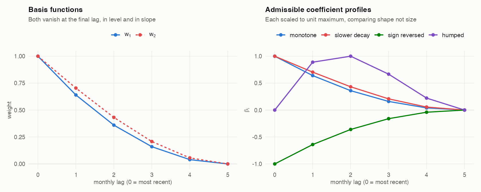{#fig-almon}## Model Overview```{r model-table}#| label: tbl-models#| tbl-cap: "Estimated specifications. All BMIDAS-GIGG variants use the Almon restriction and 6 monthly lags."tibble(Model =c("GIGG-SV-trend", "GIGG-SV", "GIGG", "PCA-MIDAS", "DFM"),Trend =c("random walk, PC prior", "none", "none", "none", "random walk"),`Observation volatility`=c("stochastic, PC prior", "stochastic, PC prior","homoskedastic", "homoskedastic", "stochastic"),`Lag treatment`=c("Almon", "Almon", "Almon", "principal components","state-space aggregation"),Shrinkage =c("GIGG", "GIGG", "GIGG", "GIGG on components, no sparsification", "none")) %>%kable()```We test 3 BMIDAS-GIGG variants which form a nested sequence of model components. GIGG-SV-trend includes a stochastic trend and stochastic volatility $(h_t,g_t)$, GIGG-SV drops the trend $(\tau_t = \bar{\tau})$, and GIGG drops both.Two models from outside the framework serve as comparators.**PCA-MIDAS** takes the unrestricted MIDAS design of every monthly lag available at a given release round and replaces it with its leading 4 principal components, recomputed at every round and every estimation window on that window's data alone. The components are extracted from the correlation matrix, because the design mixes percentage changes with standardised survey balances and an unstandardised extraction would track whichever block carries the larger variance. No trend and no stochastic volatility are applied. The approach is the factor-MIDAS of @marcellino2010factor, which extracts principal components from a ragged-edge monthly panel and regresses the quarterly target on them, and it is closely related to the daily-frequency factor constructions of @andreou2013should.We do not sparsify the component loadings. Doing so was tested and it degenerates. Group sparsification is a statement about which indicators enter, and once the regressors are principal components there are no indicator groups left to select.**DFM** is the Bayesian dynamic factor model of the Federal Reserve Bank of New York [@nyfednowcast], following @antolindiaz2024 and in the tradition of @banbura2013nowcasting. Similar to the full BMIDAS-GIGG model, it estimates a random-walk trend in mean, and stochastic volatility, however for both the factor and the idiosyncratic innovations. Additionally, it includes estimation of a discrete outlier term which @antolindiaz2024 have shown to significantly improve computational stability when outliers are contained in the data set, as well as improve nowcasting performance during crisis times. The DFM frameworks largest departure from the MIDAS framework is that it estimates the model at the lowest available frequency, here the monthly frequency, and uses the joint model over indicators and the target to interpolate any missing data at time of estimation with the system. While convenient for drawing inference on unobservable targets such as monthly GDP, the previous literature has shown that whether the DFM or MIDAS framework dominates, is often a factor of the available time-series length (often the DFM requires many more observations in order to enable accurate inference on unknown states) as well as whether the data generating process for the target is truly sparse or dense. In the latter case, it has been shown (@giannone2021economic) that factor and dynamic factor models can outperform shrinkage methods, while in the former case, estimating with shrinkage priors can outperform (additionally mutli-step ahead forecasts are often better with the full system DFM models compared to MIDAS models). Quarterly aggregation follows the Mariano-Murasawa weighting. It is estimated on the same 11 indicators and filtered through the same release calendar, so the information sets are identical by construction.# Core results {#sec-core}The evaluation covers 74 quarters from 2008Q1, with 31 quarters of training data before the first nowcast. Subsamples are the global financial crisis to the end of 2009, a tranquil period from 2010 to 2019, and the pandemic period from 2020. Quarters whose outturn is available only as a flash estimate are used as conditioning information.Three scores are reported. Write $y_t$ for the outturn, $\hat{y}_t$ for the predictive mean and $F_t$ for the predictive distribution function at quarter $t$.The root mean squared forecast error evaluates the point forecast only,$$\mathrm{RMSFE} = \sqrt{\tfrac{1}{T}\textstyle\sum_{t=1}^{T}\left(y_t - \hat{y}_t\right)^2 }.$$ {#eq-rmsfe}The continuous ranked probability score evaluates the whole density and reduces to the absolute error when the forecast is a point mass,$$\mathrm{CRPS}_t = \int_{-\infty}^{\infty}\left(F_t(z) - \mathbf{1}\{z \ge y_t\}\right)^2 dz .$$ {#eq-crps}The tail-weighted quantile score is a weighted sum of pinball losses over a grid of quantiles $\alpha$, with weights that emphasise the tails,$$\mathrm{WQS}_t = \sum_{\alpha} v(\alpha)\left(\alpha - \mathbf{1}\{y_t < F_t^{-1}(\alpha)\}\right)\left(y_t - F_t^{-1}(\alpha)\right),\qquad v(\alpha) = \left(2\alpha - 1\right)^2 .$$ {#eq-wqs}All 3 are negatively oriented, so lower is better throughout. The CRPS and the WQS are proper scoring rules in the sense of @gneiting2007strictly, so they are minimised in expectation by the true predictive distribution. The RMSFE rewards only the central tendency, which is why a model can improve on it while worsening the density.## Accuracy across the release cycle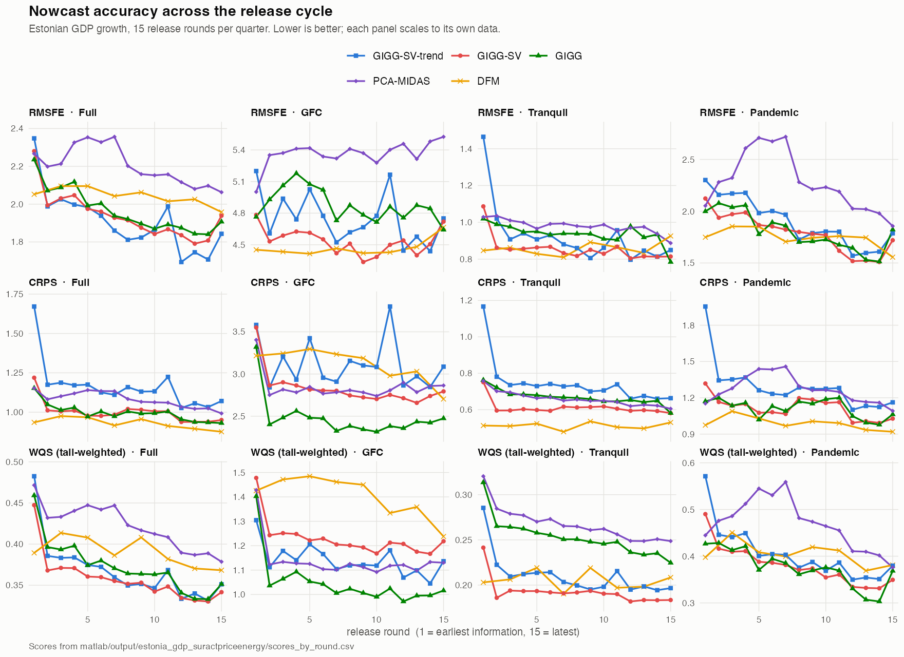{#fig-scores-core}```{r core-scores}#| label: tbl-core#| tbl-cap: "Scores averaged over release rounds. Lower is better."sub_scores %>%filter(spec %in% CORE, subsample %in%c("Full","GFC","Tranquil","Pandemic")) %>%select(spec, subsample, rmsfe, crps, wqs) %>%pivot_longer(c(rmsfe, crps, wqs), names_to ="metric") %>%mutate(metric =recode(metric, rmsfe ="RMSFE", crps ="CRPS", wqs ="WQS"),value =round(value, 3)) %>%pivot_wider(names_from = subsample, values_from = value) %>%arrange(factor(metric, levels =c("RMSFE","CRPS","WQS")),factor(spec, levels = CORE)) %>%rename(Model = spec, Metric = metric) %>%kable()``````{r dm-table}#| label: tbl-dm#| tbl-cap: "Scores relative to the GIGG benchmark. Values below 1 indicate an improvement and are shown in bold. Significance is from the Diebold-Mariano test with the Harvey-Leybourne-Newbold correction, on the same loss differentials the toolbox uses, with * p<0.10, ** p<0.05, *** p<0.01. Bare stars mark significant improvements and stars in parentheses mark significant deteriorations."dm <-d("dm_vs_benchmark.csv")# The toolbox convention stars improvements only. Reporting deteriorations unmarked would# be misleading here, because several are significant at well below the 1% level.# They are marked in parentheses.sig <-function(p) ifelse(is.na(p), "", ifelse(p <0.01, "***", ifelse(p <0.05, "**",ifelse(p <0.10, "*", ""))))fmt <-function(ratio, pval) { mark <-sig(pval)ifelse(is.na(ratio), "",ifelse(ratio <1,paste0("<strong>", sprintf("%.3f", ratio), mark, "</strong>"),paste0(sprintf("%.3f", ratio), ifelse(mark =="", "", paste0("(", mark, ")")))))}dm %>%filter(spec %in% CORE, subsample %in%c("Full","GFC","Tranquil","Pandemic")) %>%mutate(cell =fmt(ratio, pval),metric =recode(metric, rmsfe ="RMSFE", crps ="CRPS", wqs ="WQS")) %>%select(spec, subsample, metric, cell) %>%pivot_wider(names_from = subsample, values_from = cell) %>%arrange(factor(metric, levels =c("RMSFE","CRPS","WQS")),factor(spec, levels = CORE)) %>%rename(Model = spec, Metric = metric) %>%kable(escape =FALSE)```Before turning to the differences between models, note the feature they share. In @fig-scores-core every score on average declines as the release round advances. This is the minimum one should require of a nowcasting exercise as it indicated that the indicators carry information about the target and that the release calendar orders that information in a coherent way (and that the correlation structure to the target behaves in a somewhat linear way). A flat or rising profile may indicate that the data are uninformative or that the calendar is misspecified.Three results stand out.First, the ordering of the 3 GIGG variants differs between the point forecast and the density, and the Diebold-Mariano tests in @tbl-dm show the two comparisons carry very different weight. On the point forecast, GIGG-SV improves significantly on the homoskedastic GIGG in the crisis subsample, at a ratio of 0.930 with p below 0.01, and in the tranquil period, at 0.913 with p below 0.01. Over the full sample the point-forecast differences among the 3 are not significant.On the density the ranking reverses and the reversal is significant. GIGG-SV-trend is worse than GIGG on the continuous ranked probability score over the full sample, at a ratio of 1.167 with p below 0.01, and worse again in the crisis subsample at 1.258. GIGG-SV is indistinguishable from GIGG over the full sample, at 1.003 with p of 0.78, but significantly worse in the crisis subsample at 1.142. A homoskedastic model produces bands of uniform width, and over a sample containing one very large observation this turns out to be a better probabilistic description for that outturn than a model that widens its bands only after the fact. Adding the trend on top costs accuracy on both criteria and is the least attractive of the 3.Second, the dynamic factor model attains the lowest continuous ranked probability score over the full sample, but the margin over GIGG is not significant, at a ratio of 0.939 with p of 0.46. Its advantage is concentrated in the tranquil period, where the ratio of 0.746 is significant at the 1% level, and it reverses in the crisis subsample, where it scores 1.275 against GIGG.The mechanism is visible in the decomposition reported in the [appendix](#sec-appendix-dfm). The model's stochastic volatility paths are close to constant, and its random-walk trend spans a range of only 0.022 to 0.030 percentage points over 26 years. Both crises are absorbed almost entirely by the discrete outlier component, which is a multiplicative scale on the innovation variance. That scale sits at 1 in 319 of 321 months and fires exactly twice, at 2008Q4 with a multiple of 4.6 and at 2020Q3 with a multiple of 3.6. The factor model therefore handles the crisis episodes by inflating variance at two points rather than by tracking the level, and its cycle correspondingly picks up less of the variation in growth than the MIDAS models do, resulting in worse overall RMSFE. This is a different mechanism from the one the GIGG variants use, and it is why the factor model looks strong on a density score in quiet periods and weak in the crisis.Third, PCA-MIDAS is the weakest specification, and unlike the differences among the GIGG variants this one is unambiguous. It is worse than GIGG on every metric in every subsample, and significantly so at the 1% level throughout, with a full-sample point-forecast ratio of 1.121. The Almon restriction and the principal-components reduction impose different structures. The Almon polynomial restricts the lag profile within each indicator, as @fig-almon illustrates, whereas principal components impose a common low-rank structure across indicators and lags and discard indicator-specific timing. On this panel the former is clearly the more useful restriction.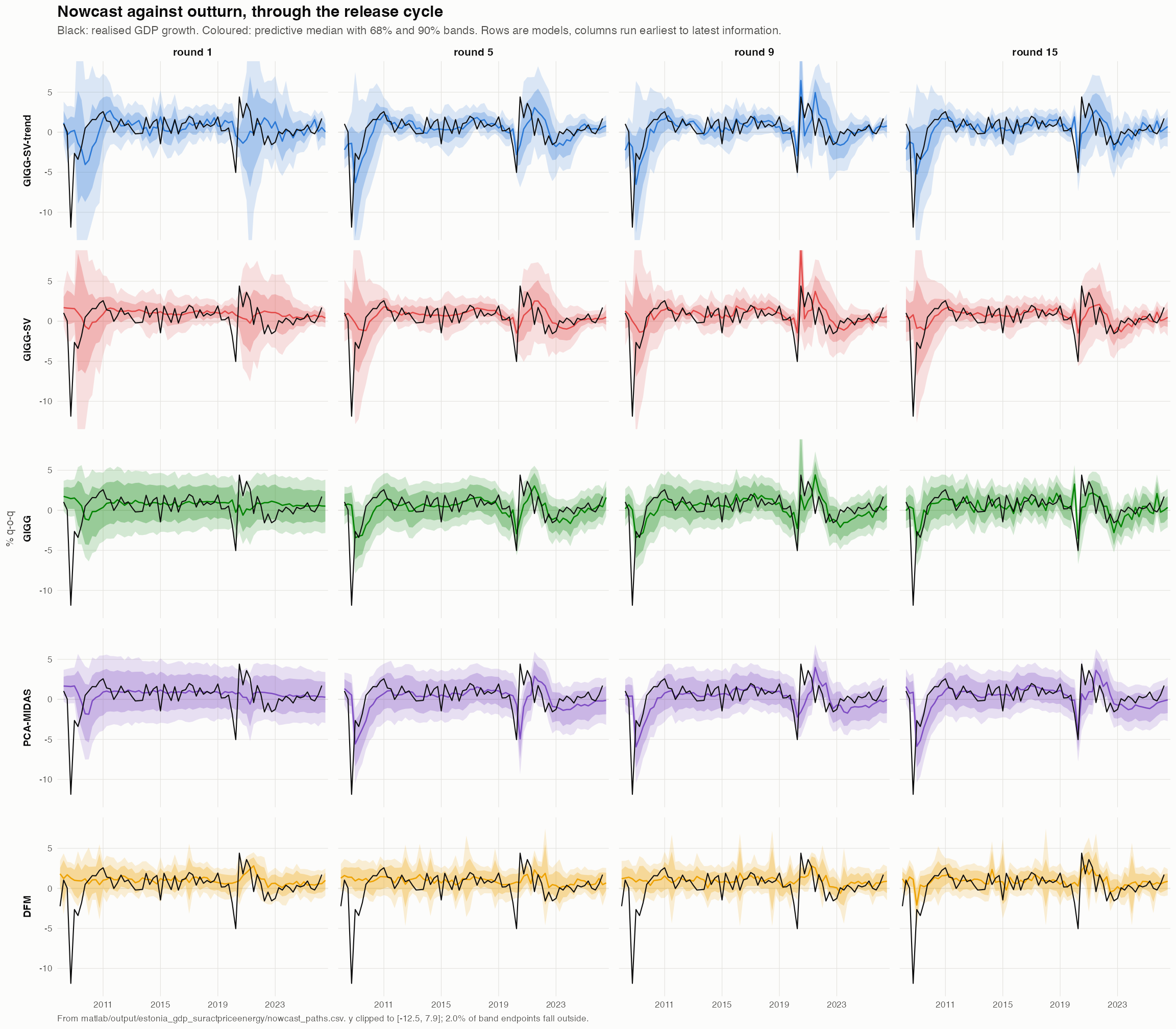{#fig-paths-core}@fig-paths-core shows the source of the score differences. All 5 models track the tranquil period closely and all 5 miss the 2008Q4 and 2020Q2 troughs. The differences between models are differences in how much uncertainty they attach to those misses and therefore how much the conditional mean is able to adjust.A feature of @fig-paths-core is worth drawing out.```{r band-table}#| label: tbl-bands#| tbl-cap: "Mean width of the 90% predictive interval, in percentage points, by release round."paths <-d("nowcast_paths.csv")paths %>%filter(spec %in% CORE, release_round %in%c(1, 3, 5, 9, 15)) %>%mutate(width = q95 - q05) %>%group_by(spec, release_round) %>%summarise(width =round(mean(width), 2), .groups ="drop") %>%pivot_wider(names_from = release_round, values_from = width,names_prefix ="round ") %>%arrange(factor(spec, levels = CORE)) %>%rename(Model = spec) %>%kable()```Uncertainty narrows as information accrues, which is the density counterpart of the score profile noted above. For the 4 MIDAS-family specifications the 90% interval contracts by between a fifth and a quarter between the first and the last round. The dynamic factor model is the exception. Its interval is both much narrower throughout and essentially flat across the cycle, moving from 4.38 to 4.35 percentage points. A model whose predictive uncertainty does not respond to the arrival of 3 additional months of hard data is not learning from the release calendar in the way the others are, and this is the same limitation that flatters its density scores. The PCA-MIDAS interval is the widest of the MIDAS family at every round, which alongside its point-forecast performance is the second reason to prefer the Almon restriction on this panel.## Trend, cycle and volatility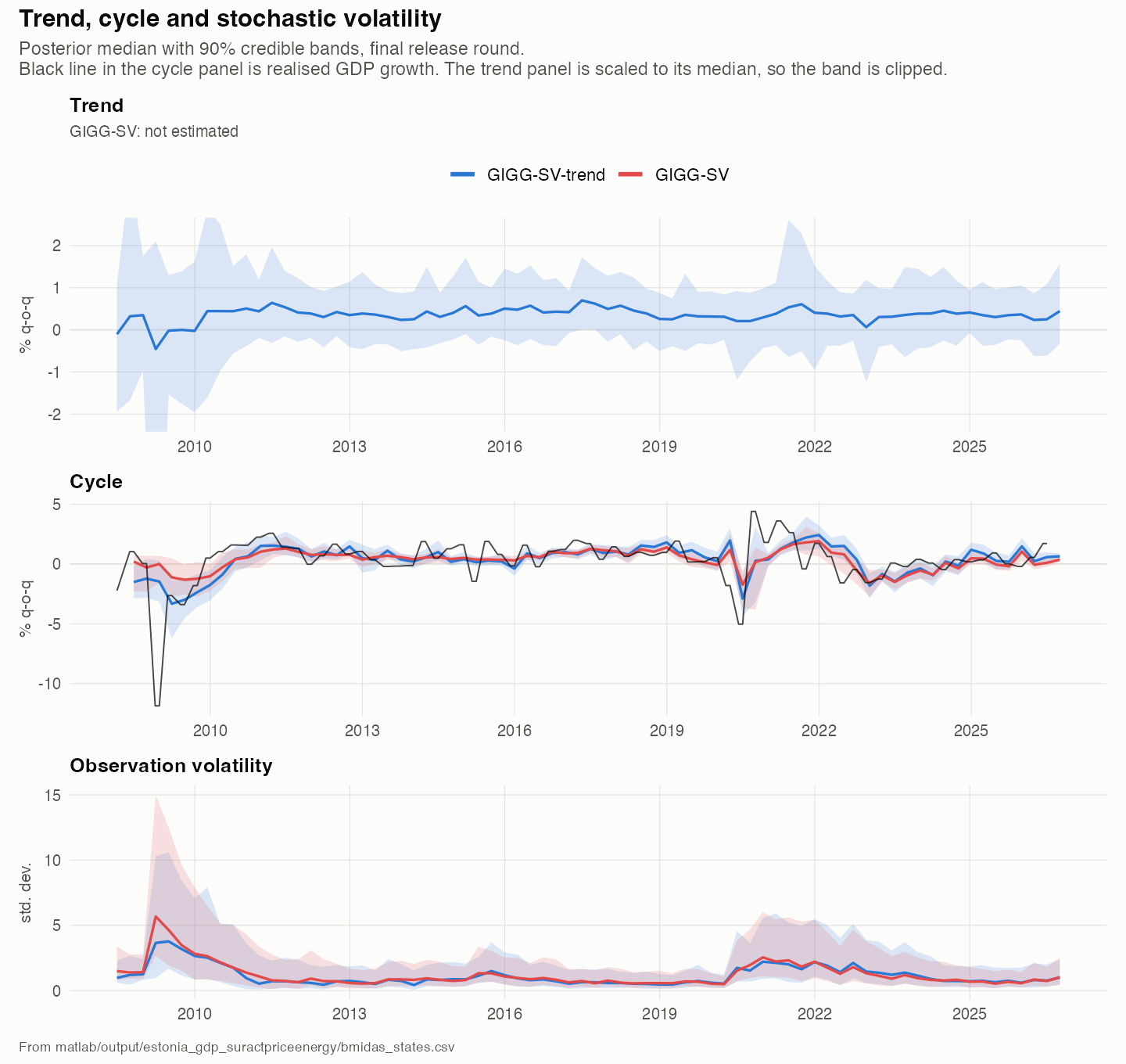{#fig-trend-core}The trend estimated by GIGG-SV-trend is close to constant at approximately 0.4% per quarter over the entire sample, with a credible band that never excludes a flat trend after 2011. This is consistent with the score evidence, where dropping the trend costs little on the point forecast, however improves density nowcasts because it allows to more flexibly model the uncertainty propagation.The cycle carries essentially all of the variation and the two models agree on it closely. The observation volatility rises sharply in 2008 and 2009, falls to a low and stable level through the 2010s, and rises again through 2020 to 2022 without approaching the crisis peak. GIGG-SV assigns systematically higher volatility than GIGG-SV-trend in the crisis episode, which is the expected consequence of removing the trend. Variation that the trend would otherwise absorb is reallocated to the variance of the observation equation.## Inclusion probabilities {#sec-inclusion}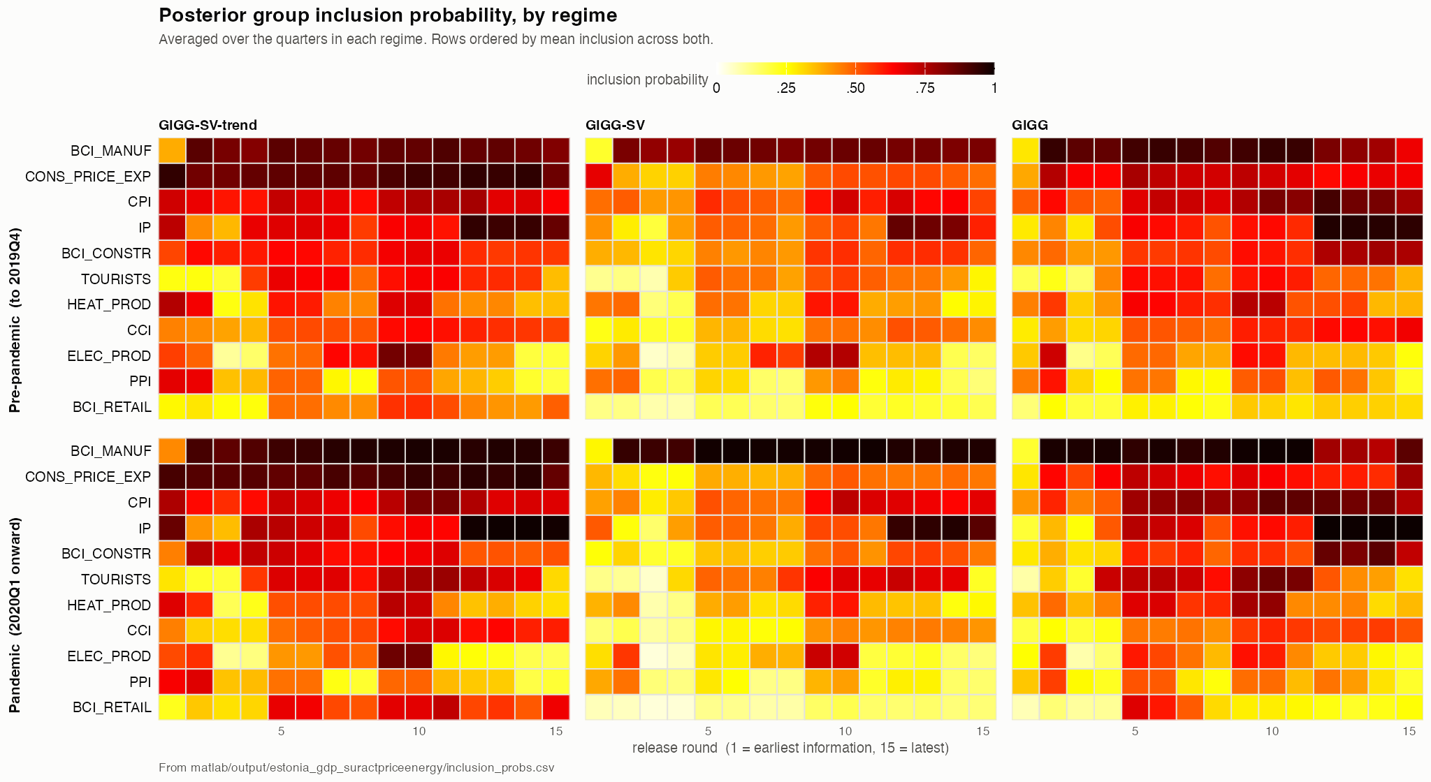{#fig-incl-core}```{r incl-table}#| label: tbl-incl#| tbl-cap: "Group inclusion probabilities at the final release round, full sample."incl %>%filter(spec %in%c("GIGG-SV-trend","GIGG-SV","GIGG"), subsample =="Full", release_round ==15) %>%mutate(prob =round(prob, 2)) %>%select(spec, indicator, prob) %>%pivot_wider(names_from = spec, values_from = prob) %>%arrange(desc(`GIGG-SV`)) %>%rename(Indicator = indicator) %>%kable()```As indicated above, we use a sparsification algorithm proposed in @kohns2025midas in order to identify which indicator over the nowcast cycle influences the nowcasts the most. The result of applying the sparsification algorithm is a number for every nowcast period for each indicator between 0 and 1 (hence, we often refer to it in the paper as an inclusion probability). The closer this number gets to 1, the more important that indicator is in forming the nowcast.The 3 BMIDAS-GIGG variants agree on which indicators matter. Industrial production and manufacturing confidence carry the highest probabilities at the final release round, and the consumer price index and consumer price expectations follow. Energy production and tourism are selected least often. This is a coherent reading for an economy in which manufacturing dominates the goods-export base.The pattern across the release cycle is more informative than the level. At early rounds, when no hard activity data are available, the survey and price groups carry the entire signal. Industrial production enters only from the rounds at which its first month becomes observable, and its probability then rises monotonically. The model reallocates weight from soft to hard information as the latter arrives, which is the behaviour the group structure was designed to produce.Interestingly, there is fairly little difference in the inclusion probabilities before and during the pandemic, whereas for the UK data nowcasting application in @kohns2025midas, there was a clear difference variable importance pre- to during the pandemic. This may suggest that Estonia's economy wasn't majorly affected by Covid in the sense of which economic drivers affect GDP growth most.In line with our previous paper, we find that there is clear evidence of sparsity, and that it varies over the release cycle. Especially when industrial production is sufficiently available, we see that this indicator received most weight while other variables are more heavily shrunk and therefore receive lower inclusion probability. This may also explain the superior performance in mean predictions of the MIDAS models over the DFM model which per modeling assumption assumes that the signal of the data is dense. Interestingly, we see that the signal sparsity clearly depends on whether SV and or the trend are modeled.## Live nowcast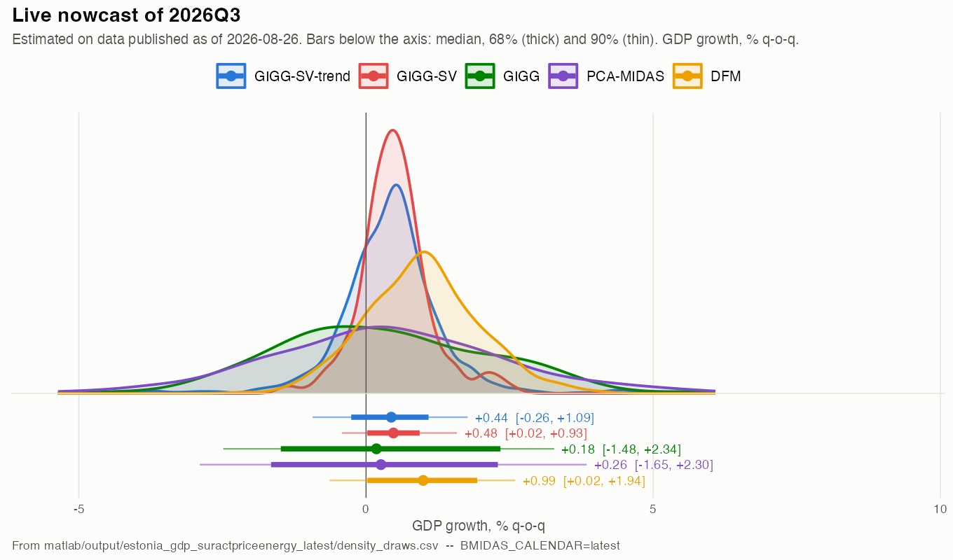{#fig-live-core}@fig-live-core reports nowcasts for 2026Q3 conditioned on all data published to date. The BMIDAS variants are estimated on the live calendar and therefore observe a single information set rather than a sequence of rounds. GIGG-SV places the median at 0.48% with a 60% interval from 0%-0.9% growth. In line with the above discussion, we find the interval larger for the GIGG-SV-trend and for the GIGG model, however the medians fairly closely agree. The dynamic factor model is more optimistic at plus 0.99% at the median, however with larger uncertainty.# Extending the dataset {#sec-extending}## Financial market dataThe core panel contains no financial information. Financial market data are the only series available with no publication delay, and their usefulness in mixed-frequency models is established [@andreou2013should]. Hence, one hypothesis is that the financial data may meaningfully improve nowcasts in the early nowcast rounds.Five series are added from the European Central Bank Data Portal. These are the EURO STOXX 50 index, the 3-month Euribor rate, the spread of the euro area 10-year benchmark bond yield over that rate, the United States dollar to euro exchange rate, and the Estonian lending rate to non-financial corporations. Rates enter in first differences and prices in percentage changes. The spread enters in levels.The timing convention deserves a comment. The series enter as monthly averages of daily observations, so a month's value is complete only at month end. They therefore carry a publication delay of zero but sit one slot behind the survey balances, which are published on the 23rd of each month. This is truthful for a monthly average and it also forgoes the main advantage of the data. A month-to-date average would make this the most timely block in the panel rather than the second most timely (which we leave to future research).## Foreign activityApproximately 46% of Estonian goods exports go to Finland, Sweden, Latvia and Germany. Foreign demand is summarised by a single export-weighted index of harmonised industrial confidence in those 4 economies, taken from Eurostat and seasonally adjusted at source.```{r foreign-weights}#| label: tbl-weights#| tbl-cap: "Export weights for the foreign activity index, from Statistics Estonia partner shares."d("foreign_diagnostics.csv") %>%mutate(across(c(mean_share_pct, weight), ~round(.x, 3))) %>%select(Country = country, `Share of goods exports, per cent`= mean_share_pct,Weight = weight) %>%kable()```Weights are fixed at the mean partner share over the full period for which Statistics Estonia publishes them. A time-varying weight would have to be lagged to remain consistent with real time and would rewrite the historical index at every vintage (hence, also left for future iterations of this project).The harmonised surveys are taken from Eurostat rather than from the OECD, because the OECD mirror of the same series runs one month behind. Foreign industrial production is available but is not used, because it carries the same two-month delay as Estonian industrial production and therefore is unlikely to improve the early rounds where the core panel is weakest.## Results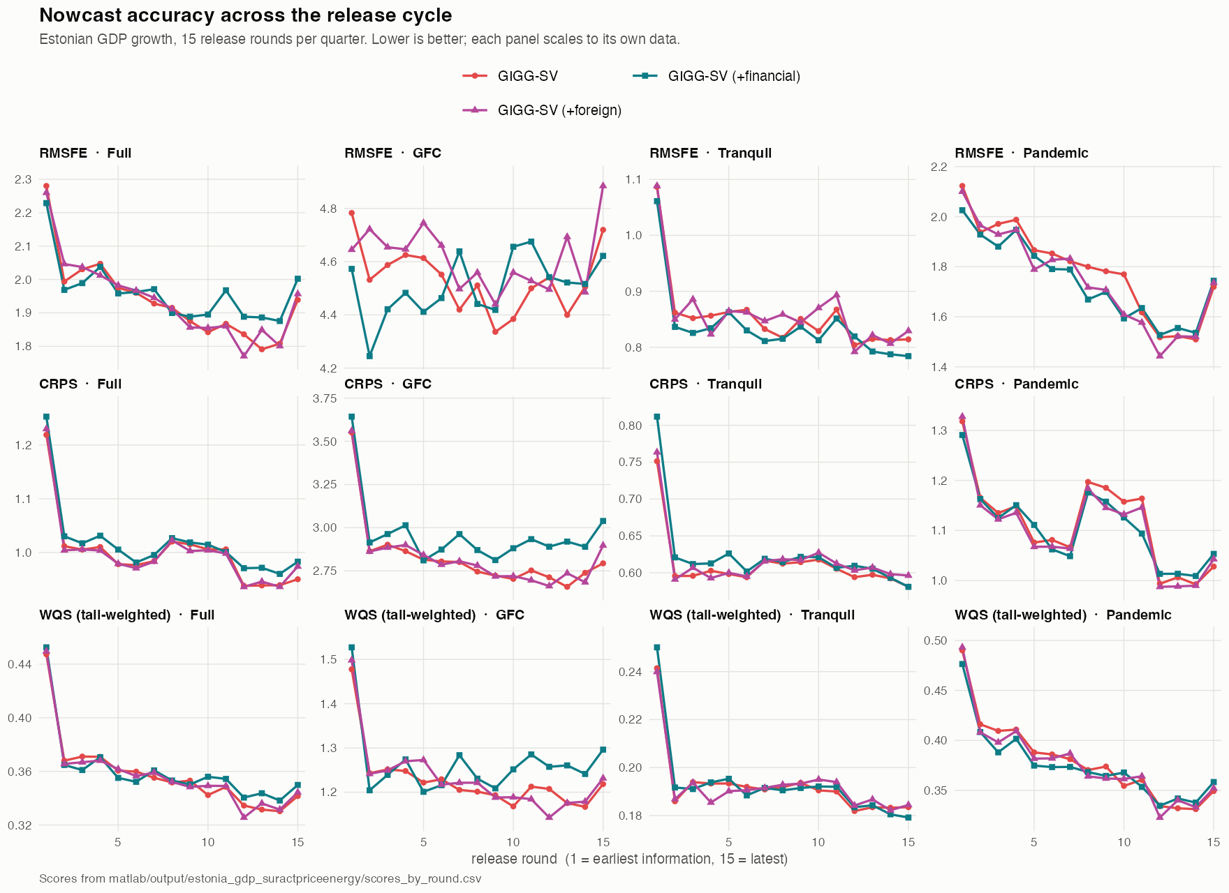{#fig-scores-panels}```{r panel-scores}#| label: tbl-panels#| tbl-cap: "GIGG-SV across indicator panels, scores averaged over release rounds."sub_scores %>%filter(spec %in% PANELS, subsample %in%c("Full","GFC","Tranquil","Pandemic")) %>%select(spec, subsample, rmsfe, crps) %>%pivot_longer(c(rmsfe, crps), names_to ="metric") %>%mutate(metric =toupper(metric), value =round(value, 3)) %>%pivot_wider(names_from = subsample, values_from = value) %>%arrange(factor(metric, levels =c("RMSFE","CRPS")), factor(spec, levels = PANELS)) %>%rename(Panel = spec, Metric = metric) %>%kable()```Neither extension improves the full-sample score significantly. The differences in @tbl-panels are within the Monte Carlo variation of the estimation procedure. The informative variation lies across release rounds rather than in the averages.Financial data improve the earliest rounds and worsen the latest. Full-sample root mean squared error at round 1 falls from 2.280 to 2.229 when the financial block is added, and at round 15 it rises from 1.939 to 2.002. The mechanism is visible in the inclusion probabilities. At round 1 the financial block occupies the top 3 positions, with the term spread at 0.62, the exchange rate at 0.52 and the 3-month rate at 0.52, ahead of every survey balance. Financial variables substitute for hard data that has not yet arrived and muddy the signal once it has.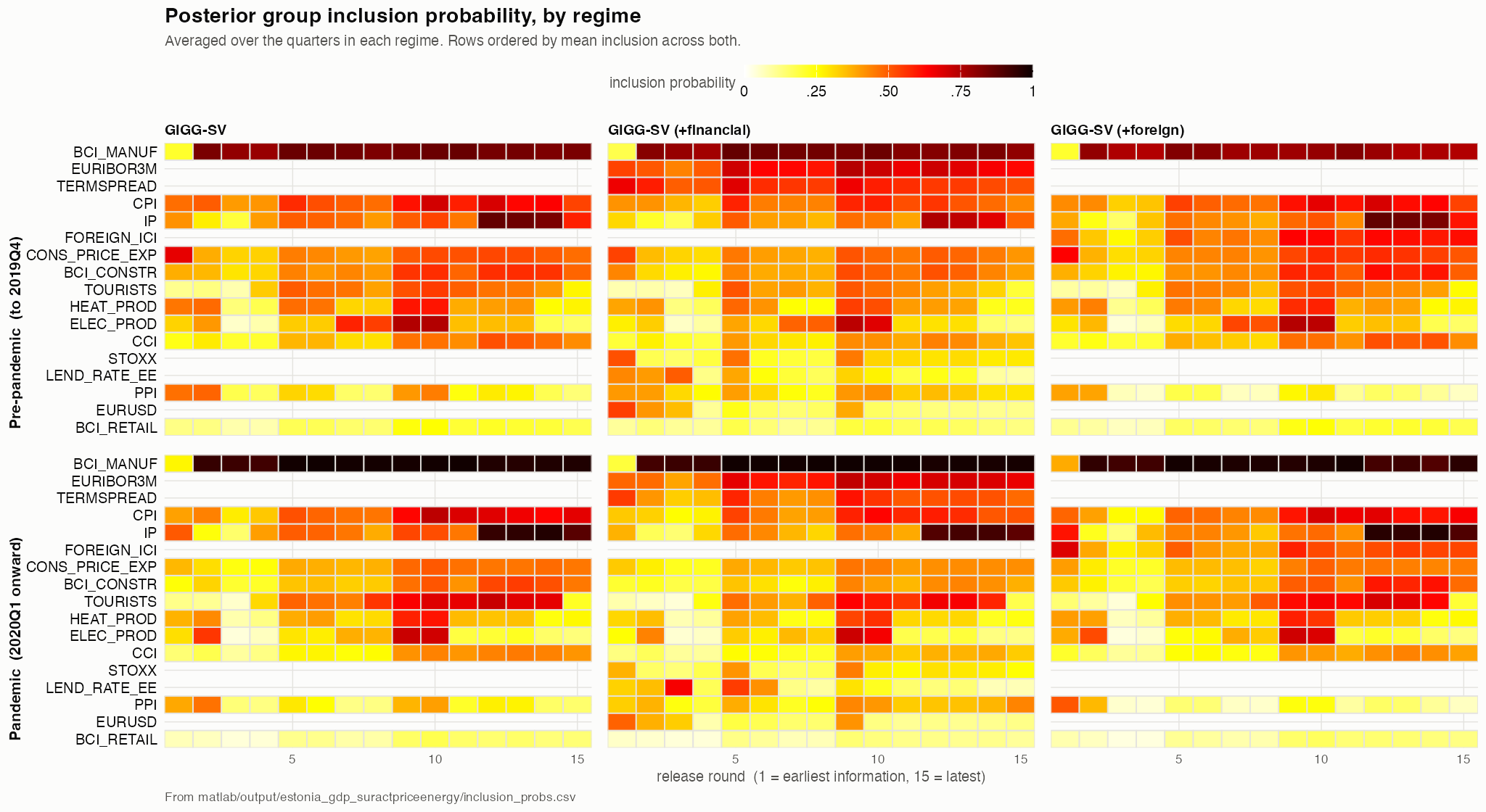{#fig-incl-panels}Foreign activity does not help on any subsample and is the weakest of the 3 panels in the crisis period, at `r val("GIGG-SV (+foreign)","GFC","rmsfe")` against `r val("GIGG-SV","GFC","rmsfe")` for the core panel. The index is selected when it is available, at an inclusion probability of 0.55 and second rank of 12 at round 1.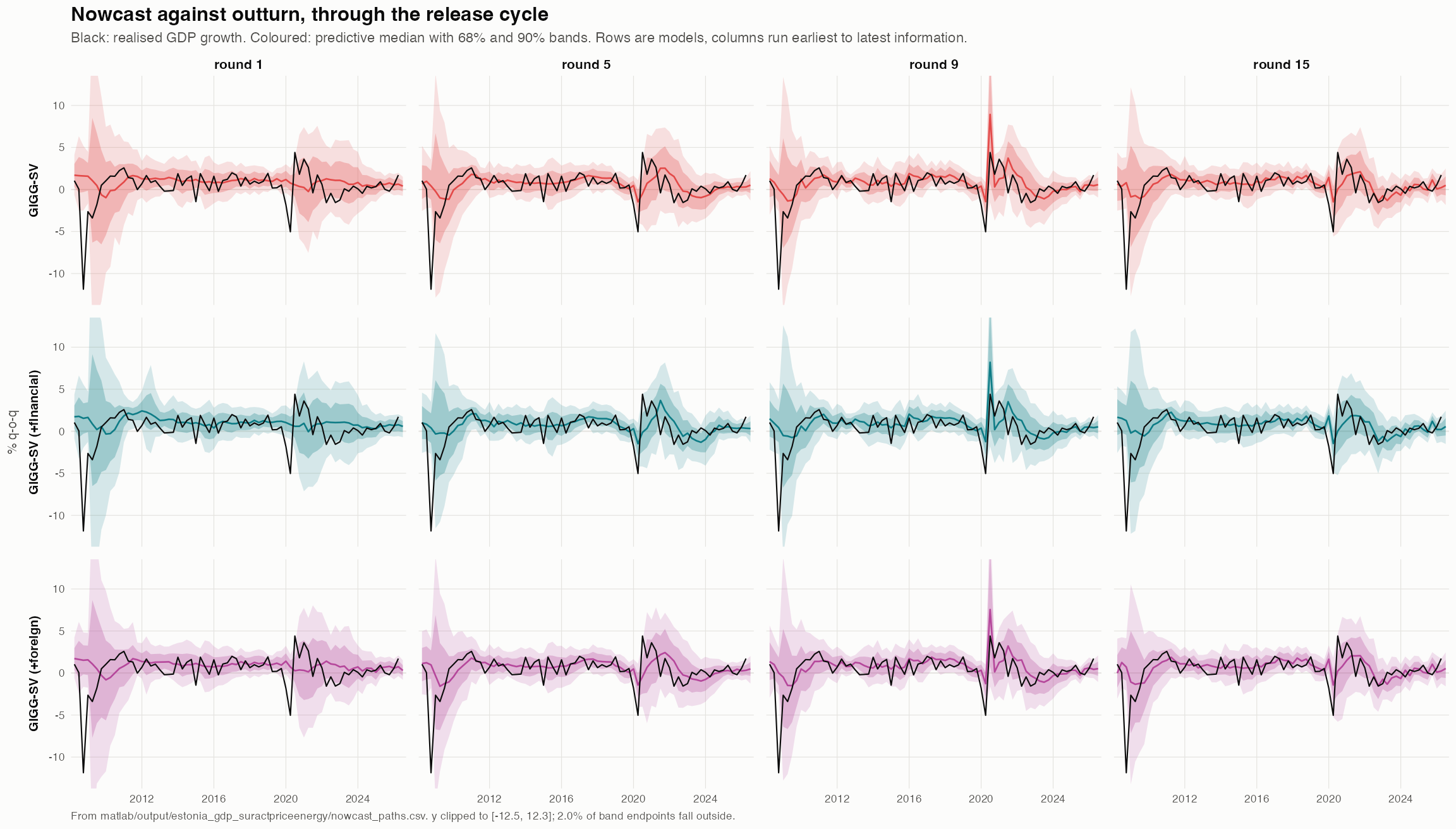{#fig-paths-panels}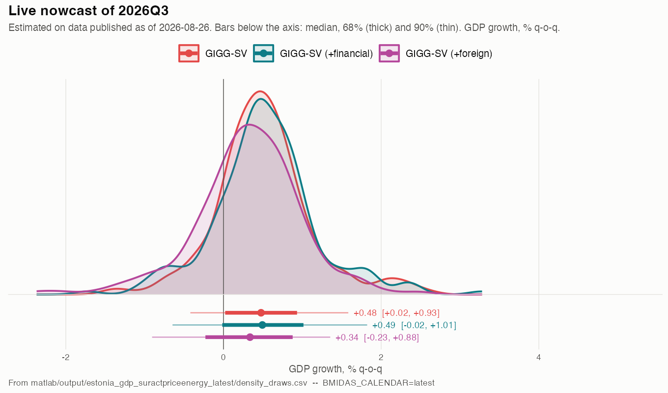{#fig-live-panels}In line with the results, the live nowcasts in @fig-live-panels don't differ meaningfully across panels.# SummaryIn this case study, we have applied the BMIDAS-GIGG toolbox proposed by @kohns2025midas applied to a new data source for nowcasting real GDP growth of Estonia. This note is intended to serve as a summary of the main methodology both for data collection and nowcast models which will be made openly available and updated in real time with each data update for Estonia. The hope is that this will improve transparency in modelling and data assumptions for nowcasting aggregate economic activity.The results show that the BMIDAS-GIGG models provide good fit to Estonian data where the GIGG-SV (stochastic volatility in the observation equation) provides a good balance between fit and parsimony. The models also improve significantly over commonly used competitors, the DFM and the PCA-MIDAS method.Certaintly there are many improvements we can make on the breadth of data as well as modelling assumptions. If you have any comments, suggestions or questions, do please feel free to reach out to me. I summarise some planned work for this project below.# Future extensions**Calibration and skewness.** The scores reported here summarise the predictive density by its distance from a realisation. They do not establish whether the densities are calibrated. Probability integral transforms and their tail behaviour would establish this directly [@gneiting2007strictly]. The evidence in @sec-core that a homoskedastic model attains the best crisis-period continuous ranked probability score suggests that the symmetric volatility specification is not capturing the shape of the predictive distribution during downturns. Asymmetry in the conditional distribution of growth is a plausible missing feature.**Financial data in the variance rather than the mean.** Financial variables improve the early nowcast rounds and degrade the late ones when they enter the conditional mean. Their established role in the literature on growth at risk is in the conditional variance and in the lower quantiles. Allowing them to load on the volatility state or on a skewness parameter, rather than on the mean, is a more natural use of what they carry.**Panel extension to Latvia and Lithuania.** The 3 Baltic economies many similarities a common set of external shocks and are individually short of data. A panel specification with partial pooling across countries would address the sample length problem identified above directly, rather than by discarding the crisis episode.**Non-standard data sources.** Internet search data improve nowcasts early in a quarter, before conventional indicators become available [@kohns_nowcasting_2022], which is precisely where the models here are weakest. Card payment records, electricity load and port traffic are further candidates with short publication delays.# How to cite {.unnumbered}This case study carries Google Scholar citation metadata in the page header, so it is indexed and citable in the same way as a working paper. Please cite the case study itself when you use the dataset, the release calendar or the results, and cite @kohns2025midas for the underlying methodology and @bmidasgigg for the estimation code. The same entry is regenerated automatically at the foot of the page.``` bibtex@online{kohns2026, author = {Kohns, David}, title = {Nowcasting {Estonian} {GDP} with {Bayesian} {MIDAS}}, date = {2026-08-26}, series = {Case Studies in Bayesian Nowcasting}, publisher = {Aalto University}, url = {https://davkoh.github.io/case-studies/03_estonia_nowcast/index.html}, urldate = {yyyy-mm-dd}}```In text: Kohns, D. (2026). *Nowcasting Estonian GDP with Bayesian MIDAS*. Case Studies in Bayesian Nowcasting. Aalto University. <https://davkoh.github.io/case-studies/03_estonia_nowcast/index.html>Because the case study is updated as new data arrive, please record the access date, and where the exact vintage matters, cite the date shown as *Modified* at the top of the page.# Appendix {.unnumbered}## Dynamic factor model decomposition {#sec-appendix-dfm .unnumbered}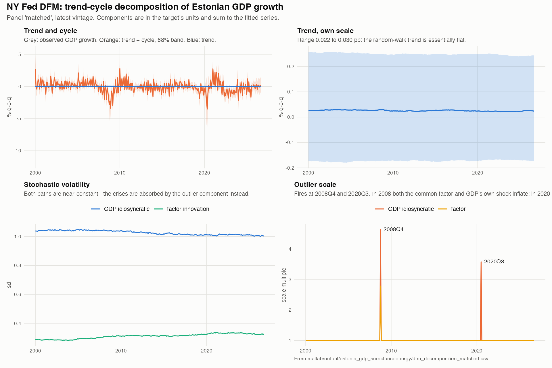{#fig-dfm-decomp}@fig-dfm-decomp supports the reading of the factor model given in @sec-core. The random-walk trend is flat to 3 decimal places. Both stochastic volatility paths, on the common factor and on the target's own innovation, are close to constant across 26 years. The crisis episodes are handled instead by the discrete outlier scale in the lower right panel, which multiplies the innovation standard deviation and is exactly 1 everywhere except at 2008Q4 and 2020Q3. In 2008 both the common factor and the target's own shock inflate. In 2020 only the target's own shock does, which is consistent with a shock that hit measured Estonian output without a corresponding common movement in the monthly indicators.The consequence for the comparison in @tbl-dm is that the factor model is close to homoskedastic between the two spikes. Its density is well calibrated in quiet periods, which is where its significant continuous ranked probability score advantage lies, and poorly suited to the crisis quarters, where it scores worse than the homoskedastic GIGG.# Original computing environment {.unnumbered}```{r session}#| code-fold: truesessionInfo()```# References {.unnumbered}


